AVR Development Board

I like to explore different instruction sets during my Computer Architecture course - typically x86-64, ARMv7, ARMv8 and AVR. For the latter, I thought it would be fun to have a small cheap development board that the students could experiment with, so I designed one.

The board uses an 8-bit Atmel AT90USB162 processor since it requires minimal external components, comes with a factory programmed USB bootloader so no additional programmer is required, and can implement USB devices such as single key keyboards and mice.

AVR Development Board

All the Eagle CAD, Gerber and placement files, along with the BOM, are available on github along with a couple of simple code examples that use AVR-GCC and Gerd’s AVR assembler (gavrasm).

Ada Lovelace

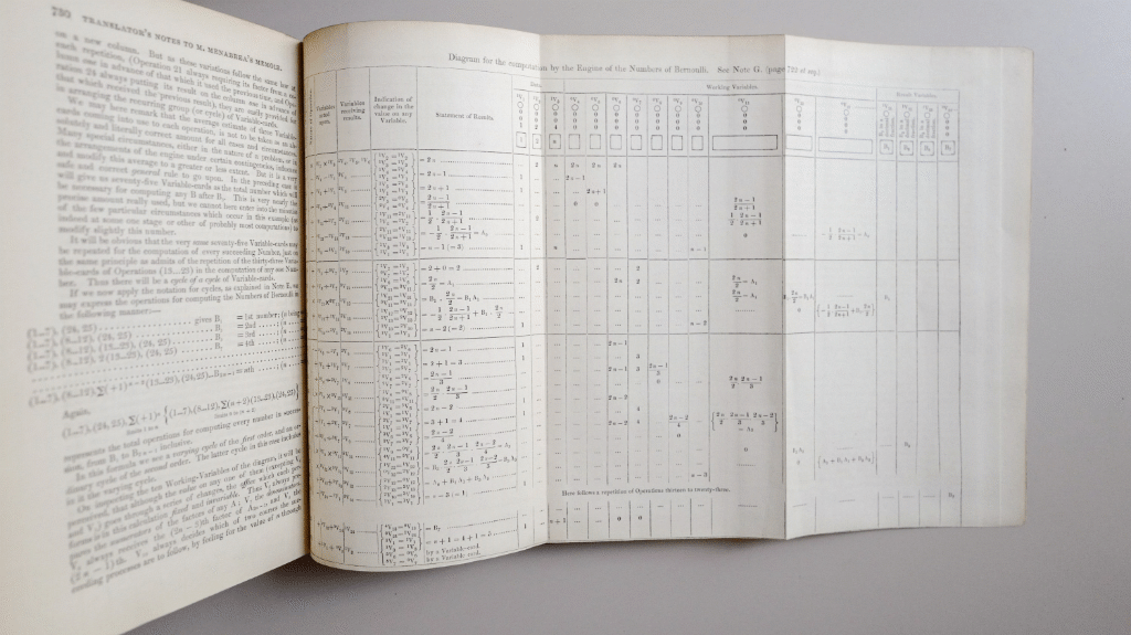
Ada Lovelace’s ‘Notes’ contained the first published computer program. More of a trace than an actual listing, it used an iterative algorithm to calculate Bernoulli numbers.

Sketch of the Analytical Engine

Here is the recreated algorithm in Julia. Ada’s original didn’t describe conditions for the repetition of operations 13 to 23, and it wasn’t clear how the array of result variables would actually be populated on the Analytical Engine. However, everything else is pretty much how her program was originally described (apart from fixing Ada’s bug in operations 4 and 24).

N = 10

v1 = BigInt(1)
v2 = BigInt(2)
v3 = BigInt(1)

v20 = fill(Rational{BigInt}(0), N)

while v3 <= N

    v7 = 0
    v13 = 0

    global v3

    # 1
    v4 = v5 = v6 = v2 * v3

    # 2
    v4 = v4 - v1

    # 3
    v5 = v5 + v1

    # 4
    v11 = v4 // v5

    # 5
    v11 = v11 // v2

    # 6
    v13 = v13 - v11

    # 7
    v10 = v3 - v1

    if v3 > 1

        # 8
        v7 = v2 + v7

        # 9
        v11 = v6 // v7

        # 10
        v12 = v20[1] * v11

        # 11
        v13 = v12 + v13

        # 12
        v10 = v10 - v1

        while v10 > 0

            # 13
            v6 = v6 - v1

            # 14
            v7 = v1 + v7

            # 15
            v8 = v6 // v7

            # 16
            v11 = v8 * v11

            # 17
            v6 = v6 - v1

            # 18
            v7 = v1 + v7

            # 19
            v9 = v6 // v7

            # 20
            v11 = v9 * v11

            # 21
            v12 = v20[v3 - v10] * v11

            # 22
            v13 = v12 + v13

            # 23
            v10 = v10 - v1

        end

    end

    # 24
    v20[v3] = v20[v3] - v13

    # 25
    v3 = v1 + v3

end

println()

for i in 1:N
    println(string(i, ": ", v20[i]))
end

println()

The results, converting to current notation (Ada’s program calculates B2n), are:

    B2 = 1/6
    B4 = -1/30
    B6 = 1/42
    B8 = -1/30
    B10 = 5/66
    B12 = -691/2730
    B14 = 7/6
    B16 = -3617/510
    B18 = 43867/798
    B20 = -174611/330

An 8-bit Manchester SSEM Simulator

I sometimes give seminars on the history of computing machines and like to use an Elm simulation of an 8-bit version of the Manchester Small-Scale Experimental Machine (SSEM). The one below is useable and there is a full page version here.

It has a memory of 32 8-bit words, an 8-bit accumulator and a 5-bit program counter. Unlike the original it doesn’t increment the program counter before executing the instruction so is a bit easier to describe and program.


The instruction set and encoding is the same as the original machine.

Inst. Description Encoding
JMP S Jump to address at S 000*****
JRP S Jump to program counter + value at S 100*****
LDN S Load and negate value at S into accumulator 010*****
STO S Store contents of accumulator at S 110*****
SUB S Subtract number at S from accumulator 101*****
CMP S Skip next instruction if accumulator is negative 011*****
STP Stop 111*****