Probability and Computing, Oxford 2018-19
Lectures
Table of Contents
- Lecture 1: A randomised algorithm for string equality
- Lecture 2: Min-cut contraction algorithm
- Lecture 3: The secretary problem and the prophet inequality
- Lecture 4: Linearity of expectations
- Lecture 5: Derandomisation
- Lecture 6: Further applications of linearity of expectations
- Lecture 7: Markov’s and Chebyshev’s inequalities
- Lecture 8: Chernoff bounds
- Lecture 9: Applications of Chernoff bounds
- Lecture 10: Martingales and stopping times
- Lecture 11: The Azuma-Hoeffding inequality
- Lecture 12: Applications of the Azuma-Hoeffding inequality
- Lecture 13: Markov chains: 2SAT and 3SAT
- Lecture 14: Markov chains and random walks
- Lecture 15: The Monte Carlo method
- Lectures 16-17: Mixing time
- Lecture 18: Lovász Local Lemma
- Lecture 19: Interactive proofs
- Lecture 20: Online algorithms - Paging
Lecture 1: A randomised algorithm for string equality
Why randomised algorithms?
Randomised algorithms make random choices. How can this help? The simple reason is that for a well-designed randomised algorithm, it is highly improbable that the algorithm will make all the wrong choices during its execution.
The advantages of randomised algorithms are:
- simplicity
- randomised algorithms are usually simpler than their deterministic counterparts
- efficiency
- they are faster, use less memory, or less communication than the best known deterministic algorithm
- dealing with incomplete information
- randomised algorithms are better in adversarial situations
Although there is a general consensus that randomised algorithms have many advantages over their deterministic counterparts, it is mainly based on evidence rather than rigorous analysis. In fact, there are very few provable cases in which randomised algorithms perform better than deterministic ones. These include the following:
- we will see an example (string equality) in which randomised
algorithms have provably better communication complexity than
deterministic algorithms
- for the similar problem of equality of multivariate polynomials, we know good randomised algorithms but no polynomial-time deterministic algorithm
- randomised algorithms provide provably better guarantees in online algorithms and learning
We have no rigorous proof that randomised algorithms are actually better than deterministic ones. This may be either because they are not really better or because we don’t have the mathematical sophistication to prove it. This is one of the outstanding open problems in computational complexity.
String equality
- String equality problem
Alice has a binary string \(a\) and Bob has a binary string \(b\), both of length \(n\). They want to check whether their strings are the same with minimal communication between them.
The straightforward method is for Alice to transmit her string to Bob who performs the check and informs Alice. This requires a communication of \(\Theta(n)\) bits. There is a better way to do it, which is based on the following reduction.
- Alice and Bob create two polynomials out of their strings: \(f(x)=\sum_{i=0}^{n-1} a_i x^i\) and \(g(x)=\sum_{i=0}^{n-1} b_i x^i\).
- In doing so, they reduce the string equality problem to the problem of checking equivalence of \(n\)-degree univariate polynomials, because the polynomials are the same if and only if they have the same coefficients.
- Checking equivalence of polynomials
Given two (univariate) polynomial \(f(x)\) and \(g(x)\) of degree \(n\), check whether they are the same.
- It helps to think that the degree of these polynomials is large (say in the billions)
- Think also of the more general problems in which the two polynomials:
- may not be in expanded form: e.g. \(f(x)=(x-3)(x^3-2x+1)^3-7\)
- may have multiple variables: e.g. \(f(x)=x_1^7(x_1^3+x_2^4)^2+2x_2\)
- Idea for algorithm
Select a large random integer \(r\) and check whether \(f(r)=g(r)\).
- Immediate question
How large \(r\) should be to achieve probability \(\epsilon\) of answering incorrectly?
- clearly there is a tradeoff between the range of \(r\) and the probability of error
- note the asymmetry (one-sided error): if the polynomials are the same, the algorithm is always correct
- if the polynomials are not the same, the algorithm returns the wrong answer exactly when \(r\) is a root of the polynomial \(f(x)-g(x)\)
- for a univariate nonzero polynomial of degree at most \(n\), there are at most \(n\) such roots1. If we select \(r\) to be a random integer in \(\{1,100n\}\), the probability of error is at most \(1/100\)
- Running time?
Note that the intermediate results of the computation may become very large. Since the degree is \(n\), \(f(r)\) may need \(\Omega(n\log n)\) bits. This is because the value of the polynomial can be as high as \(\Omega(n^n)\).
- would it not be better to transmit the original string instead of \(f(r)\)?
- the answer is no, because there is a clever way to reduce the size of numbers: do all computations in a finite field \(F_p\), for some prime \(p\geq 100n\)
- Algorithm
Here is an algorithm that implements this idea:
Select a prime \(p\) larger than \(100n\) and a random integer \(r\in \{0,\ldots,p-1\}\). Check whether
\begin{align*} f(r)=g(r) \pmod p. \end{align*}Using this algorithm, Alice and Bob can solve the string equality problem.
- Alice sends to Bob \((r, f(r) \pmod p)\). Bob checks whether \(f(r)=g(r) \pmod p\) and announces the result
- only \(O(\log n)\) bits are sent (optimal among all algorithms)
- the running time of this algorithm is polynomial in \(n\) (in fact linear, up to logarithmic factors)
- the argument for correctness is similar as above; we only replaced
the field of reals with \(F_p\)
- first notice that if the polynomials are equal, the algorithm is always correct
- otherwise, \(f(x)-g(x)\) is a nonzero polynomial of degree at most \(n\)
- but a polynomial of degree \(n < p\) has at most \(n\) roots in \(F_p\). Therefore the probability of an incorrect result is at most \(n/p\leq 1/100\)
- why do we need \(p\) to be prime? Because if \(p\) is not prime, a polynomial of degree \(n\) may have more than \(n\) roots. For example, the second-degree polynomial \(x^2-1\) has four roots \(\mod 8\)
- Loose ends
- Can we find a prime number efficiently? Yes, by repeatedly selecting
a random integer between say \(100n\) and \(200n\) until we find a
prime number
- we can check whether a number \(q\) is prime in time polynomial in \(\log q\)
- there are many prime numbers: roughly speaking, a random integer \(q\) is prime with probability approximately \(1/\ln q\) (Prime Number Theorem)
- Is probability \(1/100\) sufficient?
- we can increase the parameter \(100n\) to get a better probability; if we replace it with \(1000n\) the probability will drop to \(1/1000\)
- there is a much better way: run the test \(k\) times, with independent numbers \(r\). This will make the probability of error \(1/100^k\) (why?)
- in retrospect, and with this amplification of probability in mind, it is better to run the original test with a prime number \(p\) between \(2n\) and \(4n\) to achieve one-sided probability of error at most \(1/2\), and repeat as many times as necessary to achieve the desired bound on error
- We have seen that Alice and Bob can verify the equality of two \(n\)-bit strings by communicating \(O(\log n)\) bits. This is the best possible for randomised algorithms (why?). On the other hand, every deterministic algorithm requires \(n\) bits (why?).
- Can we find a prime number efficiently? Yes, by repeatedly selecting
a random integer between say \(100n\) and \(200n\) until we find a
prime number
Recap of useful ideas
- fingerprinting
- verify properties by appropriate random sampling
- useful trick: perform calculations modulo a prime number to keep the numbers small
- probability amplification
- run many independent tests to decrease
the probability of failure
- for one-sided error, we usually design algorithms with probability of error \(1/2\). Using probability amplification, we can easily decrease it to any desired probability bound
Further topics
- we can extend string equality to string matching (i.e. given two strings \(a\) and \(b\) check whether \(b\) is a substring of \(a\)), a very useful application. The obvious way is to check whether \(b\) appears in the first, second and so on position of \(a\). The clever trick is to find a way to combine the evaluation of the associated polynomials in an efficient way (check out the Karp-Rabin algorithm).
- it is not hard to extend the algorithm for checking polynomial identities to polynomials of multiple variables. The only difficulty is to argue about the number of roots of multi-variate polynomials (check out the Schwartz-Zippel lemma).
- applications that use efficient checking of polynomials come from unexpected domains. The perfect matching problem is such an example. The problem asks whether a given graph has a perfect matching, i.e., a set of disjoint edges that cover all vertices. The question is equivalent to whether the determinant of the Tutte matrix of the graph is not the zero polynomial (check out Tutte matrix).
Sources
- Mitzenmacher and Upfal, 2nd edition, Section 1.1
- Lap Chi Lau, L01.pdf (page 6)
- Nick Harvey, Lecture1Notes.pdf (page 3)
- James Lee, lecture1.pdf (page 1)
Lecture 2: Min-cut contraction algorithm
We will see now a strikingly simple randomised algorithm for a non-trivial graph problem.
Min-cut contraction algorithm
- The min-cut problem
Given a graph \(G(V,E)\), find a partition of the nodes into two non-empty parts in a way that minimises the number of edges from one part to the other.
- A cut of a graph \(G(V,E)\) is a non-empty subset of nodes \(S\subsetneq V\). The size of the cut is the number of edges from \(S\) to \(V\setminus S\).
- A mincut is a cut of minimum size
- Other algorithms
We can reduce this problem to the \(s-t\) maxflow-mincut problem to get a polynomial-time deterministic algorithm. Here we discuss a faster algorithm.
- Karger’s idea
Select a random edge of the graph and contract it. Most likely the new graph has the same mincut. Keep contracting random edges until the graph becomes small enough to compute the mincut directly
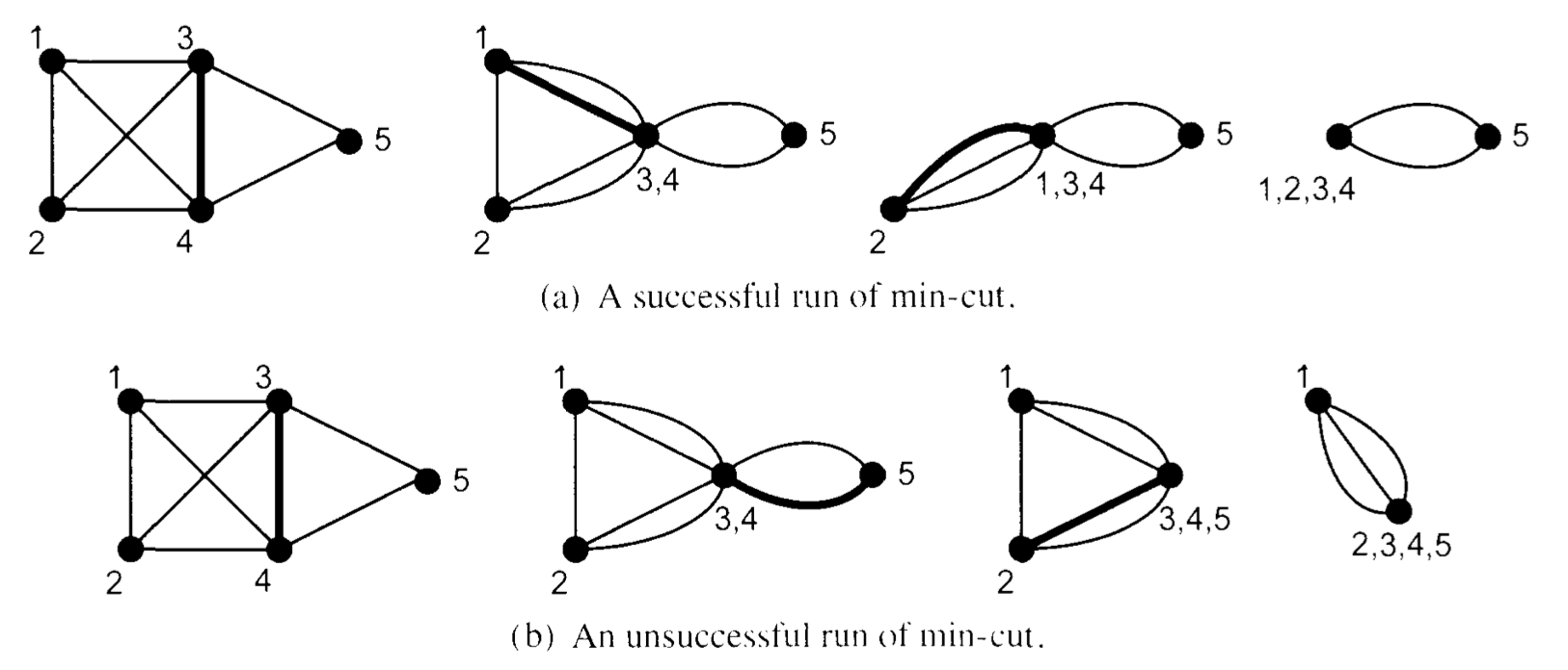
- note that the result of a contraction is in general a multigraph with self loops. We remove the loops but we leave all copies of the edges.
- Analysis
Fix a mincut \(S\). What is the probability that it will survive the first edge contraction?
- let \(k\) be the size of mincut \(S\)
- therefore the number \(m\) of edges of the multigraph is at least \(k n/2\) (Why?)2
- the probability that an edge of \(S\) is selected is \(k/m\), which is at most \(2/n\)
- the probability that \(S\) survives the first contraction is at least \(1-2/n=(n-2)/n\)
What is the probability that the mincut \(S\) will survive all contractions until only two nodes remain?
\begin{align*} \frac{n-2}{n} \frac{n-3}{n-1} \frac{n-4}{n-2}\cdots \frac{2}{4} \frac{1}{3}=\frac{2}{n(n-1)} \end{align*}- thus the probability that the contraction algorithm will be incorrect is at most \(1-\frac{2}{n(n-1)}\leq 1-\frac{2}{n^2}\)
this may seem very close to 1, but if we run the contraction algorithm \(n^2\) times and keep the best result, the probability that it will not return a mincut (in fact, the particular mincut \(S\)) will drop to 3
\begin{align*}\left(1-\frac{2}{n^2}\right)^{n^2} \leq \left(e^{-\frac{2}{n^2}}\right)^{n^2} = e^{-2} < \frac{1}{2} \end{align*}
Therefore we have:
Theorem: If we repeat the contraction algorithm \(n^2\) times, the probability that it will find a minimum cut is at least \(1/2\).
- Running time
The obvious running time is \(O(n^4)\) because we can implement every execution in \(O(n^2)\) time and we do \(n^2\) executions. This is not faster than the obvious maxflow-mincut computation, but with a little bit of effort we can significantly improve the running time of the contraction algorithm.
- this can be improved substantially if we notice that the probability that the cut \(S\) survives decreases faster as the graph becomes smaller
- to take advantage of this, we stop the contractions earlier – say when the graph has size \(r=r(n)\) – and switch to another mincut algorithm
- the probability of success becomes \(r(r-1)/n(n-1)\) and we need to repeat it only \(O(n^2/r^2)\) times to achieve probability of success at least \(1/2\)
- on the other hand, we must take into account the execution time of the algorithm we switch to when the graph reaches size \(r\)
- which algorithm should we switch to? But of course the same algorithm (recursion)
- Algorithm
Here is a variant of the above idea due to Karger and Stein:
Recursive-Contract(G)
- if n ≤ 6 use brute-force
- else repeat twice and return the best result
- G’ = Contract(G, \(n/\sqrt{2}\))
- Recursive-Contract(G’)
Contract(G, r)
- repeat until the graph has \(r\) nodes
- select a random edge and contract it
See the original paper “A new approach to the minimum cut problem” for details.
The running time of this algorithm is \(O(n^2 \log^3 n)\).
- Number of mincuts
As an extra bonus of the analysis of the contraction algorithm, we get that every graph has at most \(n(n-1)/2\) mincuts. Why? Show also that this is tight by finding a graph that has exactly \(n(n-1)/2\) mincuts.
Sources
- Mitzenmacher and Upfal, 2nd edition, Section 1.5
What is a randomised algorithm?
A randomised algorithm \(A(x,r)\) is a deterministic algorithm with two inputs. Informally, we say that \(A(x,r)\) computes a function \(f(x)\), when for a random $r\,$: \(A(x,r)=f(x)\) with significant probability.
The class Randomised-Polynomial-time (RP) consists of all languages \(L\) for which there exists a deterministic algorithm \(A(x,r)\) with running time a polynomial \(p(\cdot)\) in the length of \(x\), such that for \(r\) with \(|r|\leq p(|x|)\) and for every \(x\):
- if \(x\in L\), \(A(x,r)\) accepts for at least half of the \(r\)’s
- if \(x\not\in L\), \(A(x,r)\) rejects for all \(r\)’s.
We view this as a randomised algorithm because when we provide the algorithm with a random \(r\), it will accept with probability at least \(1/2\), when \(x\in L\), and probability \(1\), when \(x\not\in L\).
- Note the asymmetry between positive and negative instances. When an RP algorithm accepts, we are certain that \(x\in L\); when it rejects, we know that it is correct with probability at least \(1/2\).
- The class co-RP is the class with the same definition with RP, but with inverse roles of “accept” and “reject”. For example, the string equality problem is in co-RP, and the string inequality problem in RP.
- The bound \(1/2\) on the probability is arbitrary; any constant in \((0,1)\) defines the same class.
- The class NP has very similar definition. The only difference is that when \(x\in L\), the algorithm accepts not for at least half of the \(r\)’s but with at least a single \(r\).
- Similarly for the class P, the only difference is that when \(x\in L\), the algorithm accepts for all \(r\).
This shows
Theorem:
\begin{align*} P \subseteq RP \subseteq NP. \end{align*}For RP algorithms, if we want higher probability of success, we run the algorithm \(k\) times, so that the algorithm succeeds for \(x\in L\) with probability at least \(1-2^{-k}\).
Besides RP, there are other randomised complexity classes. The class ZPP (Zero-error Probabilistic Polynomial time) is the intersection of RP and its complement co-RP. Note that a language in ZPP admits an RP and a co-RP algorithm. We can repeatedly run both of them until we get an answer for which we are certain. The classes RP and ZPP correspond to the following types of algorithms
- Monte Carlo algorithm (RP)
- it runs in polynomial time and has probability of success at least \(1/2\) when \(x\in L\), and its is always correct when \(x\not\in L\).
- Las Vegas algorithm (ZPP)
- it runs in expected polynomial time and it always gives the correct answer.
Arguably, if we leave aside quantum computation, the class that captures feasible computation is the BPP class:
The class Bounded-error Probabilistic-Polynomial-time (BPP) consists of all languages \(L\) for which there exists a deterministic algorithm \(A(x,r)\) with running time a polynomial \(p(\cdot)\) in the length of \(x\), such that for \(r\) with \(|r|\leq p(|x|)\) and for every \(x\):
- if \(x\in L\), \(A(x,r)\) accepts for at least \(3/4\) of the \(r\)’s
- if \(x\not\in L\), \(A(x,r)\) rejects for at least \(3/4\) of the \(r\)’s.
- Again the constant \(3/4\) is arbitrary; any constant in \((1/2, 1)\) defines the same class.
- By repeating the algorithm many times and taking the majority, we can bring the probability of getting the correct answer very close to 1.
We don’t know much about the relation between the various classes. Clearly \(RP\subseteq BPP\), because if we run an RP algorithm twice, the probability of success is at least \(3/4\), for every input. One major open problem is whether \(BPP\subseteq NP\).
Sources
- Luca Trevisan’s notes lecture08.pdf
Lecture 3: The secretary problem and the prophet inequality
The secretary problem
We want to hire a secretary by interviewing \(n\) candidates. The problem is that we have to hire a candidate on the spot without seeing future candidates. Assuming that the candidates arrive in random order and that we can only compare the candidates that we have already seen, what is the strategy to maximise the probability to hire the best candidate?
More precisely, suppose that we see one-by-one the elements of a fixed set of \(n\) distinct numbers. Knowing only that the numbers have been permuted randomly, we have to stop at some point and pick the current number. What is the strategy that maximises the probability to pick the minimum number?
We will study the strategies that are based on a threshold \(t\): we simply interview the first \(t\) candidates but we don’t hire them. For the rest of the candidates, we hire the first candidate who is the best so far (if any).
Let \(\pi\) be a permutation denoting the ranks of the candidates. Let \(W_i^t\) denote the event that the best candidate among the first \(i\) candidates appears in the first \(t\) positions. Since the permutation is random \(\P(W_i^t)=t/i\), for \(i\geq t\).
The probability that we succeed on step \(i\), for \(i>t\), is \(\P(\pi_i=1 \wedge W_{i-1}^t)\). Since the events \(\pi_i=1 \wedge W_{i-1}^t\) are mutually exclusive, we can write the probability of success as
\begin{align*} \sum_{i=t+1}^n \P(\pi_i=1 \wedge W_{i-1}^t)&= \sum_{i=t+1}^n \frac{1}{n} \frac{t}{i-1} \\ &= \frac{t}{n} \sum_{i=t+1}^n \frac{1}{i-1} \\ &= \frac{t}{n} \left(\sum_{k=1}^{n-1} \frac{1}{k} -\sum_{k=1}^{t-1} \frac{1}{k}\right) \\ &= \frac{t}{n} (H_{n-1} - H_{t-1}) \\ &\approx \frac{t}{n} \ln \frac{n}{t}. \end{align*}This achieves its maximum value \(1/e\), when \(t=n/e\).
It is not very complicated to show that there is an optimal strategy which is a threshold strategy4. Thus
Theorem: The optimal strategy for the secretary problem, as \(n\rightarrow\infty\) is to sample \(\lceil n/e\rceil\) candidates and then hire the first candidate who is best so far (if there is any). The probability that it hires the best candidate approaches \(1/e\) as \(n\rightarrow\infty\).
The prophet inequality
Let \(X_1,\ldots,X_n\) be nonnegative independent random variables drawn from distributions \(F_1,\ldots,F_n\). We know the distributions but not the actual values. We see one-by-one the values \(X_1,\ldots,X_n\) and at some point we select one without knowing the future values. This is our reward. What is the optimal strategy to optimise the expected reward?
It is easy to see that we can find the optimal strategy by backwards induction. If we have reached the last value, we definitely select \(X_n\). For the previous step, we select \(X_{n-1}\) when \(X_{i-1}\geq \E[X_n]\), and so on. The following theorem says that we can get half of the optimal reward with a threshold value.
Theorem: Let \(X_1,\ldots,X_n\) be independent random variables drawn from distributions \(F_1,\ldots,F_n\). There is a threshold \(t\), that depends on the distributions but not the actual values, such that if we select the first value that exceeds \(t\) (if there is any), the expected reward is at least \(\E[\max_i X_i]/2\).
Proof:
We will use the notation \((a)^{+}=\max(0,a)\).
Let \(q_t\) denote the probability that no value is selected, i.e., \(q_t=P(\max_i X_i \leq t)\). Therefore with probability \(1-q_t\) the reward is at least \(t\). If only one value \(X_i\) exceeds the threshold \(t\), then the reward is this value \(X_i > t\). If more than one values exceed \(t\) then the reward is one of them, the first one. To simplify, we will assume that when this happens, we will count the reward as \(t\). To make the calculation precise, let’s first define \(q_t^i=P(\max_{j\neq i} X_j \leq t)\) and observe that \(q_t^i\geq q_t\) for all \(i\).
The expected reward \(\E[R_t]\) can be bounded by
\begin{align*} \E[R_t] &\geq (1-q_t) t + \sum_{i=1}^n q_t^i \E[(X_i-t)^+] \\ &\geq (1-q_t) t + \sum_{i=1}^n q_t \E[(X_i-t)^+] \\ &= (1-q_t) t + q_t \sum_{i=1}^n \E[(X_i-t)^+]. \end{align*}On the other hand we can find an upper bound of the optimum reward as follows:
\begin{align*} \E[\max_i X_i] & =\E[t+\max_i(X_i-t)] \\ & \leq t+\E[\max_i (X_i-t)^+] \\ & \leq t+\E\left[\sum_{i=1}^n (X_i-t)^+\right] \\ & =t+\sum_{i=1}^n \E[(X_i-t)^+]. \end{align*}By selecting \(t\) such that5 \(q_t=1/2\), we see that the threshold strategy achieves at least half the optimal value.
The above theorem is tight as the following example shows: Fix some \(\epsilon>0\) and consider \(X_1=\epsilon\) (with probability 1), \(X_2=1\) with probability \(\epsilon\), and \(X_2=0\) with probability \(1-\epsilon\). Then no strategy (threshold or not) can achieve a reward more than \(\epsilon\), while the optimal strategy has expected reward \(2\epsilon-\epsilon^2\) and the ratio tends to \(1/2\) as \(\epsilon\) tends to 0.
Sources
- Luca Trevisan’s notes on the secretary problem lecture17.pdf
- Tim Roughgarden’s notes on the prophet inequality l6.pdf
Lecture 4: Linearity of expectations
Linearity of expectations
Theorem: For every two random variables \(X\) and \(Y\):
\begin{align*} \E[X+Y]=\E[X]+\E[Y]. \end{align*}In general for a finite set of random variables \(X_1,\ldots, X_n\):
\begin{align*} E\left[\sum_{i=1}^{n} X_i\right]=\sum_{i=1}^n \E[X_i]. \end{align*}Note that linearity of expectations does not require independence of the random variables!
Remark: Most uses of probability theory can be seen as computational tools for exact and approximate calculations. For example, one can do all the math in this course using counting instead of probabilistic arguments. However, the probabilistic arguments give an intuitive and algorithmically efficient way to reach the same conclusions. During this course, we will learn a few “computational tricks” to calculate exactly or to bound random variables. On the surface, they seem simple and intuitive, but when used appropriately they can be turned into powerful tools. One such trick that we have already used is “independence”. And here we learn the “linearity of expectations” trick.
Max Cut
- The Max Cut problem
Given a graph \(G(V,E)\), find a cut of maximum size, i.e., find a set of vertices \(C\subset V\) that maximises
\begin{align*} \left|\{[u,v]\,:\, u\in C, v\not\in C\}\right|. \end{align*}This is a known NP-hard problem. It is also an APX-hard problem, meaning that unless P=NP, there is no approximation algorithm with approximate ratio arbitrarily close to 1.
With respect to approximability, an optimisation problem may
- have a polynomial time algorithm
- have a PTAS (polynomial-time approximation scheme): for every
\(\epsilon>0\), there is a polynomial time algorithm that finds a
solution within a factor \(\epsilon\) from the optimum. For example,
a PTAS can have running time \(O(n^{1/\epsilon})\)
- have a FPTAS (fully polynomial-time approximation scheme): a PTAS whose running time is also polynomial in \(1/\epsilon\), for example \(O(n/\epsilon^2)\)
- be APX-hard, i.e. it has no PTAS. This does not mean that an APX-hard problem cannot be approximated at all, but that it cannot be approximated to any desired degree. For example, we will now see that Max Cut can be approximated within a factor of \(1/2\); we say that Max Cut is APX-hard because it is known than unless P=NP, there is no polynomial-time algorithm to find solutions within a factor of \(1/17\) from the optimal solution.
- Approximate algorithm for Max Cut
There are many simple polynomial-time algorithms with approximation ratio \(1/2\). Here we will discuss a randomised algorithm:
Select a random cut, i.e., every node is put in \(C\) with probability \(1/2\).
This algorithm is so simple that it produces a cut without even looking at the graph!
- Analysis
Theorem: For every graph with \(m\) edges, the above algorithm returns a cut with expected number of edges equal to \(m/2\).
Proof: Let \(C\) be the cut produced by the algorithm. We will show that the expected number of edges crossing \(C\) is \(m/2\), where \(m\) is the number of edges of the graph. Since the optimum cut cannot have more than \(m\) edges, the approximation ratio is at least \(1/2\).
Fix an edge \([u,v]\). Let \(X_{u,v}\) be an indicator random variable that takes value 1 if \([u,v]\) is in cut \(C\) and 0 otherwise.
The probability that the edge is in the cut is
\begin{align*} \P((u\in C \wedge v\not\in C) \vee (u\not\in C \wedge v\in C))=\frac{1}{2}\cdot\frac{1}{2}+\frac{1}{2}\cdot\frac{1}{2}=\frac{1}{2}. \end{align*}Therefore \(\E[X_{u,v}]=\frac{1}{2}\cdot 1+\frac{1}{2}\cdot 0=\frac{1}{2}\).
Let \(X=\sum_{[u,v]\in E} X_{u,v}\) be the size of cut \(C\). The expected number of edges \(E[X]\) in cut \(C\) is
\begin{align*} \E\left[\sum_{[u,v]\in E} X_{u,v}\right] &= \sum_{[u,v]\in E} \E[X_{u,v}] \\ &=\sum_{[u,v]\in E} \frac{1}{2} \\ &=\frac{m}{2} \end{align*}Notice the use of the linearity of expectations.
The above analysis shows that the expected cut is of size \(m/2\), but it provides no information about the probability distribution of the size of the cut. An interesting question is how many times in expectation we need to repeat the algorithm to get a cut of size at least \(m/2\).
Here is a simple way to compute such a bound. Let \(p\) be the probability that we obtain a cut of size at least \(m/2\). Then we have
\begin{align*} \frac{m}{2} = \E[X] & = \sum_{i < m/2} i \cdot \P(X=i) + \sum_{i \geq m/2} i \cdot \P(X=i) \\ & \leq \left(\frac{m}{2}-1\right)\P\left(X \leq \frac{m}{2}-1\right) + m \P\left(X \geq \frac{m}{2}\right)\\ & = \left(\frac{m}{2}-1\right)\left(1-p\right) + mp\\ & = \left(\frac{m}{2}-1\right)+\left(\frac{m}{2}+1\right)p \end{align*}We conclude that \(p \geq \frac{1}{m/2+1}\), and hence that the expected number of trials before finding a cut of size of at least \(m/2\) is at most \(m/2+1\).
- The probabilistic method
The analysis shows that in every graph there exists a cut with at least half the edges of the graph.
The statement is a typical result of the probabilistic method: show existence of a special type object by showing either that
- a random object is of the special type with non-zero probability
- the expected number of the special type objects is positive
MAX-3-SAT
- The MAXSAT problem
Given a Boolean CNF formula, find a truth assignment that maximises the number of satisfied clauses.
This is a generalisation of the SAT problem and it is NP-hard. It is also APX-hard, i.e., there is no PTAS for this problem unless P=NP.
There are interesting special versions of the problem: MAX-2-SAT, MAX-3-SAT, and in general MAX-k-SAT in which the input is a k-CNF formula. All these special cases are NP-hard and APX-hard.
- Randomised algorithm for MAX-3-SAT
The following is a simple algorithm for the MAXSAT problem.
Select a random assignment, i.e., set every variable independently to true with probability \(1/2\).
Remark: Again, this is so simple that one can hardly consider it an algorithm; it decides the output without looking at the clauses. Not all randomised algorithms are so simple, but in general they are simpler than their deterministic counterparts.
- Analysis
We will analyse the performance of the algorithm for the special case of MAX-3-SAT. A similar analysis applies to the general MAXSAT problem, and we will revisit it later when we discuss how to “derandomise” this algorithm.
Theorem: For every 3-CNF formula with \(m\) clauses, the expected number of clauses satisfied by the above algorithm is \(\frac{7}{8}m\).
Proof: Let \(\varphi=C_1\wedge\cdots\wedge C_m\) be a formula with clauses \(C_1,\ldots,C_m\). Let \(X_i\), \(i=1,\ldots,m\), be an indicator random variable of whether a random assignment satisfies clause \(C_i\) or not. The probability that \(X_i\) is \(1\) is equal to \(7/8\), because out of the \(8\) possible (and equiprobable) assignments to the three distinct variables of \(C_i\) only one does not satisfy the clause, i.e. \(\P(X_i=1)=7/8\).
From this we get \(\E[X_i]=7/8\cdot 1 + 1/8\cdot 0=7/8\) and by linearity of expectations:
\begin{align*} \E\left[\sum_{i=1}^m X_i\right] &= \sum_{i=1}^m \E[X_i] \\ &=\sum_{i=1}^m \frac{7}{8} \\ &=\frac{7}{8}m \end{align*}Note the similarity of this proof and the proof for approximating Max Cut. Interpreting this result with the probabilistic method, we see that for every 3-CNF formula there is a truth assignment that satisfies at least \(7/8\) of its clauses.
Sources
- Mitzenmacher and Upfal, 2nd edition, Section 6.2
Lecture 5: Derandomisation
Derandomisation (method of conditional expectations)
Derandomisation is the process of taking a randomised algorithm and transform it into an equivalent deterministic one without increasing substantially its complexity. Is there a generic way to do this? We don’t know, and in fact, we have randomised algorithms that we don’t believe that can be directly transformed into deterministic ones (for example, the algorithm of verifying identity of multivariate polynomials). But we do have some techniques that work for many randomised algorithms. The simpler such technique is the method of conditional expectations. Other more sophisticated methods of derandomisation are based on reducing the number of required randomness and then try all possible choices.
Derandomisation using conditional expectations
To illustrate the idea of the method of conditional expectations, suppose that we have a randomised algorithm that randomly selects values for random variables \(X_1,\ldots,X_n\) with the aim of maximising \(\E[f(X_1,\ldots,X_n)]\). The method of conditional expectations fixes one-by-one the values \(X_1,\ldots,X_n\) to \(X_1^{*},\ldots,X_n^{*}\) so that \(f(X_1^{*},\ldots,X_n^{*}) \geq \E[f(X_1,\ldots,X_n)]\). To do this, we compute
\begin{align*} X_n^{*}&=\argmax_x \E[f(X_1,\ldots,X_n)\, | \,X_n=x] \\ X_{n-1}^{*}&=\argmax_x \E[f(X_1,\ldots,X_n)\, | \, X_n=X_n^{*}, X_{n-1}=x] \\ X_{n-2}^{*}&=\argmax_x \E[f(X_1,\ldots,X_n)\, | \, X_n=X_n^{*}, X_{n-1}=X_{n-1}^{*}, X_{n-2}=x] \\ \vdots \\ X_1^{*}&=\argmax_x \E[f(X_1,\ldots,X_n)\, | \, X_n=X_n^{*}, \ldots, X_2=X_2^{*},X_1=x] \ \end{align*}to obtain successively values \(X_n^{*},\ldots,X_1^{*}\) for which \(f\) takes a value at least as big as its expectation. If we can compute the above deterministically and efficiently, we obtain a deterministic algorithm that is as good as the randomised algorithm.
In many cases, the random variables \(X_i\) are indicator variables, which makes it easy to compute the argmax expression by computing the conditional expectation for \(X_i=0\) and \(X_i=1\) and selecting the maximum.
Derandomisation of the MAXSAT algorithm
Recall the MAXSAT algorithm which simply selects a random truth assignment. We now show how to derandomise this algorithm. When we analysed the approximation ratio for MAXSAT, we did it only for MAX-3-SAT because it was simpler. But for the discussion here, it is easier to consider general CNF formulas. In general, the inductive approach for derandomising a problem with the method of conditional expectations is facilitated by an appropriate generalisation of the problem at hand.
The crucial observation is:
Lemma: For every CNF formula with clauses of sizes \(c_1,\ldots,c_m\), the expected number of clauses satisfied by a random truth assignment is \(\sum_{i=1}^m (1-2^{-c_i})\).
Proof: The probability that the \(i\) -th clause is satisfied is \(1-2^{-c_i}\), because out of the \(2^{c_i}\) truth assignments to the variables of the clause6, only one does not satisfy the clause. If \(Z_i\) is an indicator random variable that captures whether clause \(i\) is satisfied, then \(\E[Z_i]=1-2^{-c_i}\) (we used a similar reasoning when we analysed the MAX-3-SAT algorithm). We want to compute \(\E[\sum_{i=1}^m Z_i]\). With the linearity of expectations this is \(\sum_{i=1}^m \E[Z_i]=\sum_{i=1}^m (1-2^{-c_i})\).
Given this, we can design an algorithm that satisfies at least so many clauses as in the lemma. It is best illustrated by an example.
Let \(\varphi(x_1,x_2,x_3)=(x_1 \vee \overline{x}_2)\wedge (\overline{x}_1 \vee \overline{x}_3)\wedge (x_1 \vee x_2 \vee x_3)\). A random truth assignment satisfies \(1-2^{-2}+1-2^{-2}+1-2^{-3}=19/8\) clauses, in expectation.
If we fix the value of \(x_3\) to
- true
- the resulting formula is \((x_1 \vee \overline{x}_2)\wedge (\overline{x}_1)\wedge \text{true}\). A random assignment satisfies \(1-2^{-2}+1-2^{-1}+1=9/4\) clauses.
- false
- the resulting formula is \((x_1 \vee \overline{x}_2)\wedge \text{true} \wedge (x_1 \vee x_2)\). A random assignment satisfies \(1-2^{-2}+1+1-2^{-2}=5/2\) clauses.
We must have \(\frac{1}{2}\frac{9}{4}+\frac{1}{2}\frac{5}{2}=\frac{19}{8}\), which implies that the maximum of the values \(9/4\) and \(5/2\) (the two conditional expectations) must be at least \(19/8\). Indeed, \(5/2\geq 19/8\). This suggests that we set \(x_3\) to false and repeat with the resulting formula \((x_1 \vee \overline{x}_2)\wedge \text{true} \wedge (x_1 \vee x_2)\).
We can generalise this approach to every CNF formula and we can turn it into the following algorithm:
max-sat(\(\varphi(x_1 ,\ldots, x_n)\))
- Let \(c_1^1, \ldots, c_k^1\) be the sizes of all clauses containing literal \(x_n\)
- Let \(c_1^0, \ldots, c_l^0\) be the sizes of all clauses containing literal \(\overline{x}_n\)
- If \(\sum_{i=1}^k 2^{-c_i^0}\geq \sum_{i=1}^l 2^{-c_i^1}\) then set \(x_n=\) true, else set \(x_n=\) false
- Repeat for the formula \(\varphi'(x_1, \ldots, x_{n-1})\) that results when we fix \(x_n\)
Note that we simplified the comparison of the expectations for the two cases \(x_n=\text{true}\) and \(x_n=\text{false}\) to \(\sum_{i=1}^k 2^{-c_i^0}\geq \sum_{i=1}^l 2^{-c_i^1}\).
Theorem: For every 3CNF formula, the above polynomial-time deterministic algorithm returns a truth assignment that satisfies at least \(7/8\) of the clauses.
It is known that unless P=NP, this is the best approximation ratio achievable by polytime algorithms.
Derandomisation of the Max Cut algorithm
Recall the randomised algorithm for Max Cut which partitions the vertices of the graph randomly. To derandomise it, we will fix one-by-one these random choices. To do this, let \(X_i\) be an indicator random variable of whether vertex \(i\) is in the cut, and let \(c(X_1, \ldots, X_n)\) be a random variable that gives the size of the cut. The derandomisation is based on the computation of \(\E[c(X_1, \ldots, X_n) \, |\, X_i=X_i^{*},\ldots, X_n=X_n^{*}]\), which is the expected size of the cut after we fix the position of vertices \(i,\ldots,n\). An edge contributes to this expectation:
- 1, if both vertices have been fixed and are in different parts
- 0, if both vertices have been fixed and are in the same part
- \(1/2\), if at least one of the vertices has not been fixed,
from which we get the following claim.
Claim:
\begin{align*} \E[c(X_1, \ldots, X_n) | X_i=X_i^{*},\ldots, X_n=X_n^{*}] &= \sum_{[u,v]\in E} \begin{cases} 1 & \text{$u,v\geq i$ and $X_u^{*}\neq X_v^{*}$} \\ 0 & \text{$u,v\geq i$ and $X_u^{*} = X_v^{*}$} \\ \frac{1}{2} & \text{otherwise}. \end{cases} \end{align*}The algorithm then is:
max-cut(G)
- For \(i=n,\ldots,1\)
- if \(\E[c(X_1, \ldots, X_n) | X_i=1, X_{i+1}=X_{i+1}^{*},\ldots, X_n=X_n^{*}] \geq\) \(\E[c(X_1,\ldots,X_n) | X_i=0, X_{i+1}=X_{i+1}^{*},\ldots, X_n=X_n^{*}]\), fix \(X_i^{*}=1\) and put vertex \(i\) into the cut,
- otherwise, fix \(X_i^{*}=0\) and do not put vertex \(i\) into the cut.
A closer look at this algorithm shows that it is essentially the greedy algorithm: it processes vertices \(n,\ldots,1\) and for each one of them, it puts it in the part that maximises the cut of the processed vertices.
Theorem: For every graph \(G\), the above polynomial-time deterministic algorithm returns a cut of size at least half the total number of edges.
Sources
- Mitzenmacher and Upfal, 2nd edition, Sections 6.3
Pairwise independence and derandomization
Recall that random variables \(X_1,\ldots,X_n\) are independent if \[\P(X_1=a_1 \cap \cdots \cap X_n=a_n) = \P(X_1=a_1) \cdots \P(X_n=a_n)\] for all \(a_1,\ldots,a_n\).
We say that \(X_1,\ldots,X_n\) are pairwise independent if
\begin{align*} \P(X_i=a_i \cap X_j=a_j) = \P(X_i=a_i) \cdot \P(X_j=a_j), \end{align*}for \(i \neq j\).
Bits for free!
A random bit is uniform if it assumes the values 0 and 1 with equal probability. Suppose \(X_1, \ldots, X_n\) are independent uniform random bits. Given a non-empty set \(S \subseteq \{1,\ldots,n\}\), define \(Y_S = \bigoplus_{i \in S} X_i\) (where \(\oplus\) denotes exclusive or). Clearly \(\P(Y_S=1) = 1/2\) 7. Similarly, given two different non-empty sets \(S, T \subseteq \{1,\ldots,n\}\), we have for every \(i,j\in\{0,1\}\):
\begin{align*} \P(Y_S=i \wedge Y_T=j)=1/4. \end{align*}Therefore
Claim: The \(2^n-1\) random variables \(Y_S=\bigoplus_{i \in S} X_i\), where \(S\) a non-empty subset of \(\{1,\ldots,n\}\) are pairwise independent.
Note though that the \(Y_S\)’s are not fully independent since, e.g., \(Y_{\{1\}}\) and \(Y_{\{2\}}\) determine \(Y_{\{1,2\}}\).
Application: Finding max cuts
Let \(G=(V,E)\) be an undirected graph with \(n\) vertices and \(m\) edges. Recall the argument that \(G\) has a cut of size at least \(m/2\). Suppose that we choose \(C\subseteq V\) uniformly at random. Let \(X\) be the number of edges with one endpoint in \(C\) and the other in \(V \setminus C\). Then \(\E[X] = m/2\) by linearity of expectations. We conclude that there must be some cut of size at least \(m/2\).
The above existence result is not constructive—it does not tell us how to find the cut. We have seen how to derandomise this algorithm using conditional expectations. Here we see another way to derandomise the algorithm using pairwise independence.
Let \(b = \lceil\log (n+1)\rceil\) and let \(X_1, \ldots, X_b\) be independent random bits. As explained above we can obtain \(n\) pairwise independent random bits \(Y_1, \ldots, Y_n\) from the \(X_i\). Now writing \(V=\{1,\ldots,n\}\) for the set of vertices of \(G\) we take \(A=\{ i : Y_i=1\}\) as our random cut. An edge \([i,j]\) crosses the cut iff \(Y_i \neq Y_j\), and this happens with probability \(1/2\) by pairwise independence. Thus, writing again \(X\) for the number of edges crossing the cut, we have \(\E[X] \geq m/2\). We conclude that there exists a choice of \(Y_1, \ldots, Y_n\) yielding a cut of size \(\geq m/2\). In turn this implies that there is a choice of \(X_1, \ldots, X_b\) yielding a cut of size \(\geq m/2\). But now we have a polynomial-time deterministic procedure for finding a large cut: try all \(2^b=O(n)\) values of \(X_1, \ldots, X_b\) until one generates a cut of size at least \(m/2\).
Sources
- Mitzenmacher and Upfal, 2nd edition, Sections 6.3
Lecture 6: Further applications of linearity of expectations
Coupon collector’s problem
The geometric distribution
Random processes in which we repeat an experiment with probability of success \(p\) until we succeed are captured by the geometric distribution.
A random variable \(X\) is geometric with parameter \(p\) if it takes values \(1,2,\ldots\) with
\begin{align*} \P(X=n)=(1-p)^{n-1}p. \end{align*}The following properties follow from the definition or directly from the intuitive memoryless property of independent repeated experiments.
Lemma: For a geometric random variable \(X\) with parameter \(p\)
\begin{align*} \P(X=n+k \, |\, X>k) &= \P(X=n) \\ \E[X] &= \frac{1}{p} \end{align*}Coupon collector’s problem - expectation
In the coupon collector’s problem, there are \(n\) distinct coupons. Each day we draw a coupon independently and uniformly at random with the goal of selecting all \(n\) different types of coupons. The question that we are interested in is: how many days on expectation do we need to select all coupons?
Let \(X_i\) be the number of days between the time we obtain \(i-1\) distinct coupons and the time we obtain \(i\) distinct coupons. We want to compute \(\E[\sum_{i=1}^n X_i]\). Note that if we have \(i-1\) coupons, the probability of obtaining a new coupon is
\begin{align*} p_i&=\frac{n-i+1}{n}. \end{align*}We repeat the experiment until we succeed, at which point we have one more coupon and the probability drops to \(p_{i+1}\). That is, the random variable \(X_i\) is geometric with parameter \(p_i\). By linearity of expectations, we can now compute the expected number of days to collect all coupons:
\begin{align*} \E[\sum_{i=1}^n X_i] &= \sum_{i=1}^n \E[X_i] \\ &= \sum_{i=1}^n 1/p_i \\ &= \sum_{i=1}^n \frac{n}{n-i+1} \\ &= n H_n, \end{align*}where \(H_n=1+\frac{1}{2}+\cdots+\frac{1}{n}\) is the \(n\) -th Harmonic number, approximately equal to \(\ln n\).
Sources
- Mitzenmacher and Upfal, 2nd edition, Section 2.4
Randomised quicksort
Quicksort is a simple and practical algorithm for sorting large sequences. The algorithm works as follows: it selects as pivot an element \(v\) of the sequence and then partitions the sequence into two parts: part \(L\) that contains the elements that are smaller than the pivot element and part \(R\) that contains the elements that are larger than the pivot element. It then sorts recursively \(L\) and \(R\) and puts everything together: sorted \(L\), \(v\), sorted \(R\).
Randomised Quicksort selects the pivot elements independently and uniformly at random. We want to compute the expected number of comparisons of this algorithm.
Theorem: For every input, the expected number of comparisons made by Randomised Quicksort is \(2n\ln n+O(n)\).
Proof: Let \(v_1, \ldots, v_n\) be the elements of the sequence after we sort them. The important step in the proof is to define indicator random variables \(X_{i,j}\) of whether \(v_i\) and \(v_j\) are compared at any point during the execution of the algorithm. We want to estimate \(\E[\sum_{i=1}^{n-1}\sum_{j=i+1}^n X_{i,j}]\).
The heart of the proof is to compute \(\E[X_{i,j}]\) by focusing on the elements \(S_{i,j}=\{v_i, \ldots, v_j\}\) and observing that
- the algorithm compares \(v_i\) with \(v_j\) if and only if the first element from \(S_{i,j}\) to be selected as pivot is either \(v_i\) or \(v_j\).
Given that the pivot elements are selected independently and uniformly at random, the probability for this to happen is \(2/(j-i+1)\). From this and the linearity of expectations, we get
\begin{align*} E\left[ \sum_{i=1}^{n-1}\sum_{j=i+1}^n X_{i,j} \right] &= \sum_{i=1}^{n-1}\sum_{j=i+1}^n \frac{2}{j-i+1} \\ &= \sum_{i=1}^{n-1}\sum_{k=2}^{n-i+1} \frac{2}{k} \\ &= \sum_{k=2}^n \sum_{i=1}^{n-k+1} \frac{2}{k} \\ &= \sum_{k=2}^n (n-k+1) \frac{2}{k} \\ &= (n+1)\sum_{k=2}^n \frac{2}{k} - 2(n-1)\\ &= 2(n+1)\sum_{k=1}^n \frac{1}{k} - 4n \\ &= 2(n+1)H_n - 4n. \end{align*}Since \(H_n=\ln n+O(1)\), we get that the expectation is \(2n\ln + O(n)\).
Sources
- Mitzenmacher and Upfal, 2nd edition, Section 2.5
Jensen’s inequality
Another application of the linearity of expectations is a proof of Jensen’s inequality, a very general lemma and an important tool in probability theory.
Lemma: For every convex function \(f\) and every random value \(X\) with finite expectation:
\begin{align*} \E[f(X)] &\geq f(\E[X]). \end{align*}The theory of convex functions of one or more variables plays an important part in many fields and in particular in algorithms. A function is called convex if for every \(x\), \(y\), and \(\lambda\in[0,1]\): \(f(\lambda x+(1-\lambda) y)\leq \lambda f(x)+(1-\lambda) f(y)\).
Jensen’s inequality holds for every convex function \(f\), but for simplicity we will prove it only for differentiable \(f\). For differentiable functions, the definition of convexity is equivalent to: for every \(x\) and \(y\), \(f(y)\geq f(x)+f'(x)(y-x)\).
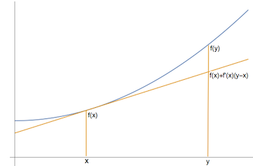
Figure 2: A convex function: \(f(y)\geq f(x)+f'(x)(y-x)\)
With this, Jensen’s inequality is a trivial application of the linearity of expectations:
Proof: Let \(\mu=\E[X]\). We then have \(f(X) \geq f(\mu)+f'(\mu)(X-\mu)\). This implies that
\begin{align*} \E[f(X)] & \geq f(\mu)+f'(\mu)(\E[X]-\mu) \\ & = f(\mu)+f'(\mu)(\mu-\mu) \\ & = f(\mu) \\ & = f(\E[X]). \end{align*}An immediate application of Jensen’s inequality is that for every random variable \(X\): \(\E[X^2]\geq (\E[X])^2\).
Sources
- Mitzenmacher and Upfal, 2nd edition, Section 2.1
Lecture 7: Markov’s and Chebyshev’s inequalities
Markov’s and Chebyshev’s inequalities
We have seen that in many cases we can easily compute exactly or approximately the expectation of random variables. For example, we have computed the expected value of the number of comparisons of Randomised Quicksort to be \(2n\ln n+O(n)\). But this is not very informative about the behaviour of the algorithm. For example, it may be that the running time of the algorithm is either approximately \(n\) or approximately \(n^2\), but never close to the expected running time. It would be much more informative if we new the distribution of the number of comparisons of the algorithm. Concentration bounds–also known as tail bounds–go a long way towards providing this kind of information: they tell us that some random variable takes values close to its expectation with high probability. We will see a few concentration bounds in this course, such as Markov’s and Chebyshev’s inequality and Chernoff’s bound. All these provide inequalities for probabilities.
Union bound
Before we turn our attention to concentration bounds, we will consider a simple bound on probabilities, the union bound. In most applications, it is not strong enough to give any useful result, but there are surprisingly many cases that the bound is useful and sometimes it is the only available tool.
Lemma [Union bound]: For any countable set of events \(E_1,E_2,\ldots\),
\begin{align*} \P(\cup_{i\geq 1} E_i)\leq \sum_{i\geq 1} \P(E_i). \end{align*}If the events \(E_i\) are mutually exclusive, the union bound holds with equality8.
Example [Ramsey numbers - lower bound]: The Ramsey number \(R(k,m)\) is the smallest integer \(n\) such that for every graph \(G\) of \(n\) vertices, either \(G\) has a clique of size \(k\) or the complement graph \(\overline{G}\) has a clique of size \(m\). For example \(R(3,3)=6\). Ramsey’s theorem, which can be proved by induction, states that \(R(k,m)\) is well defined. Of particular interest are the numbers \(R(k,k)\), and the following theorem based on the union bound is the best lower bound that we have on these numbers.
Theorem: If \(\binom{n}{k}<2^{\binom{k}{2}-1}\) then \(R(k,k)>n\). Therefore \(R(k,k)=\Omega(k 2^{k/2})\).
Proof: Consider the complete graph of \(n\) vertices and colour its edges independently and uniformly at random with two colours. If with positive probability there is no monochromatic clique of size \(k\), then \(R(k,k)>n\).
A fixed subset of \(k\) vertices is monochromatic with probability \(2^{1-\binom{k}{2}}\). There are \(\binom{n}{k}\) such subsets and, by the union bound, the probability that there exists a monochromatic clique of size \(k\) is at most \(\binom{n}{k} 2^{1-\binom{k}{2}}\). If this is less than 1, there exists a colouring that does not create a monochromatic triangle. Thus, if \(\binom{n}{k} 2^{1-\binom{k}{2}}<1\) then \(R(k,k)>n\). This proves the first part of the theorem. The second part is a simple consequence when we solve for \(n\).
Markov’s inequality
Markov’s inequality is the weakest concentration bound.
Theorem [Markov's inequality]: For every non-negative random variable \(X\) and every \(a>0\),
\begin{align*} \P(X\geq a)\leq \frac{\E[X]}{a}. \end{align*}Proof: The proof explores an idea that we have seen a few times: If \(Y\) is a 0-1 indicator variable, then \(\E[Y]=\P(Y)\). Indeed, let \(Y\) be the indicator variable of event \(X\geq a\). Observe that \(Y\leq X/a\) because
- if \(Y=1\) then \(X\geq a\)
- if \(Y=0\) then \(Y\leq X/a\), because \(X\geq 0\).
Therefore \(\P(X\geq a)=\P(Y)=\E[Y]\leq \E[X/a] = \E[X]/a\), which proves the lemma.
Although Markov’s inequality does not provide much information about the distribution of the random variable \(X\), it has some advantages:
- it requires that we only know the expected value \(\E[X]\)
- it applies to every non-negative random variable \(X\)
- it is a useful tool to obtain stronger inequalities when we know more about the random variable \(X\)
Example: Markov’s inequality is useful in turning bounds on expected running time to probability bounds. For example, the expected number of comparisons of Randomised Quicksort is \(2n\ln n+O(n)\leq 3n\ln n\), for large \(n\). Thererefore, the probability that the number of comparisons is more than \(6n\ln n\) is at most \(1/2\); more generally, the probability that the number of comparisons is more than \(3kn\ln n\) is at most \(1/k\), for every \(k\geq 1\).
Example: Let’s try to use Markov’s inequality to bound the probability of success of the randomised Max Cut algorithm. We have seen that the size \(X\) of the cut returned by the algorithm has expectation \(m/2\). What is the probability that the returned cut is at least \(m/4\)? By applying Markov’s inequality, we get that the probability is at most \(2\), a useless bound!
But here is a trick: let’s consider the number of edges that are not in the cut. This is a random variable \(Y=m-X\) whose expectation is also \(m/2\). We want to bound the probability \(\P(X\geq m/4)=\P(Y\leq 3m/4)=1-\P(Y>3m/4)\). By Markov’s inequality \(\P(Y>3m/4)\leq 2/3\), from which we get that the probability that the randomised Max Cut algorithm returns a cut of size \(X\geq m/4\) is at least \(1-2/3=1/3\). By a straightforward generalisation, we get that the probability that the randomised Max Cut algorithm returns a cut of size greater than \((1-\epsilon) m/2\) is at least \(\epsilon/(1+\epsilon)\). In particular, by taking \(\epsilon=1/m\) and using the fact that \(m\) is an integer, we get that the probability that the algorithm returns a cut of size at least \(m/2\) (i.e., greater than \((m-1)/2\)) is at least \(1/(m+1)\).
The technique of applying Markov’s inequality to a function of the random variable we are interested in, instead of the random variable itself, is very powerful and we will use it repeatedly.
Variance and moments
The \(k\)-th moment of a random variable \(X\) is \(\E[X^k]\).
The variance of a random variable \(X\) is
\begin{align*} \var[X]=\E[(X-\E[X])^2]=\E[X^2]-\E[X]^2. \end{align*}Its square root is called standard deviation: \(\sigma[X]=\sqrt{\var[X]}\).
The second equality holds because
\begin{align*} \E[(X-\E[X])^2]=\E[X^2-2X\E[X]+\E[X]^2]=\E[X^2]-2\E[X]\E[X]+\E[X]^2=\E[X^2]-\E[X]^2. \end{align*}The covariance of two random variables \(X\) and \(Y\) is
\begin{align*} \cov[X,Y]=\E[(X-\E[X])(Y-E[Y])]. \end{align*}We say that \(X\) and \(Y\) are positively (negatively) correlated when their covariance is positive (negative).
Lemma: For any random variables \(X\) and \(Y\):
\begin{align*} \var[X+Y]=\var[X]+\var[Y]+2\cov[X,Y]. \end{align*}If \(X\) and \(Y\) are independent then \(\cov[X,Y]=0\) and \(\var[X+Y]=\var[X]+\var[Y]\).
More generally, for pairwise independent random variables \(X_1\ldots,X_n\):
\begin{align*} \var\left[\sum_{i=1}^n X_i\right]=\sum_{i=1}^n \var[X_i]. \end{align*}Chebyshev’s inequality
Chebyshev’s inequality is a tail bound that involves the first two moments.
Theorem: For every random variable \(X\) and every \(a>0\),
\begin{align*} \P(|X-\E[X]|\geq a) \leq \frac{\var[X]}{a^2}. \end{align*}Proof: The proof is an application of Markov’s inequality to the (non-negative) random variable \(Y=(X-\E[X])^2\). Indeed, from the definition of \(\var[X]\) we have that \(\E[Y]=\var[X]\), and by applying Markov’s inequality we get
\begin{align*} \P((X-\E[X])^2\geq a^2)\leq \frac{\E[Y]}{a^2} = \frac{\var[X]}{a^2}, \end{align*}which proves the theorem.
Example [Binomial random variables]: We have seen that indicator random variables are very useful. An indicator random variable represents the outcome of a Bernoulli trial, which is a random experiment with two outcomes, success or failure.
A binomial random variable \(X\) with parameters \(n\) and \(p\) is the sum of \(n\) independent Bernoulli (indicator) random variables, each with probability \(p\); we write \(X\sim B(n,p)\). It follows immediately that for \(X\sim B(n,p)\),
\begin{align*} \P(X=i)=\binom{n}{i}p^i(1-p)^{n-i}. \end{align*}The expectation and variance of a binomial random variable \(X\) with parameters \(n\) and \(p\) is \(np\) and \(np(1-p)\), respectively.
We often need to estimate the probability \(\P(X\geq k)=\sum_{i=k}^n \P(X=i)=\sum_{i=k}^n \binom{n}{i}p^i(1-p)^{n-i}\). Instead of this complicated sum, we want a simple expression that approximates it. Let’s see what we get when we apply Markov’s and Chebyshev’s inequality to bound \(\P(X\geq 3n/4)\) when \(p=1/2\) (equivalent to the probability of getting more than \(3n/4\) heads when we throw a fair coin \(n\) times).
- Markov’s inequality
- \begin{align*} \P(X\geq 3n/4)\leq (n/2)/(3n/4) = 2/3 \end{align*}
- Chebyshev’s inequality
- \begin{align*} \P(X\geq 3n/4)\leq \P(|X-n/2| \geq n/4) \leq (n/4)/(n/4)^2 = 4/n. \end{align*}
Markov’s and Chebyshev’s inequalities provide some bounds on this probability, but they are not very accurate. We will see later that Chernoff’s bound gives a much better estimate.
Coupon collector’s problem - probability
In many applications, Chebyshev’s inequality is sufficient to get decent results.
Consider the coupon collector’s problem. We have seen that the time for collecting all coupons is the sum of \(n\) geometric variables \(X_i\), \(i=1,\ldots, n\), with parameters \((n-i+1)/n\) and \(\E[\sum_{i=1}^n X_i]=n H_n\).
The variance of a geometric variable with parameter \(p\) is \((1-p)/p^2\). Given that the \(X_i\)’s are independent, we have
\begin{align*} \var\left[\sum_{i=1}^n X_i\right] &=\sum_{i=1}^n \frac{n(i-1)}{(n-i+1)^2} \\ &\leq \sum_{i=1}^n \left(\frac{n}{n-i+1}\right)^2 \\ &= n^2 \sum_{i=1}^n \frac{1}{i^2} \\ &\leq \frac{\pi^2 n^2}{6}. \end{align*}With this, we can apply Chebyshev’s inequality to get
\begin{align*} \P(|X-n H_n|\geq nH_n)\leq \frac{\pi^2 n^2/6}{(n H_n)^2}=O\left(\frac{1}{\log^2 n}\right), \end{align*}which says that the probability to exceed the expectation by a factor of 2 is small. Although Chebyshev’s inequality provide a decent estimate in this case, we know much stronger concentration bounds for the coupon collector’s problem.
Sources
- Mitzenmacher and Upfal, 2nd edition, Sections 3.1
- Nick Harvey, Lecture2Notes.pdf (page 2)
- Lap Chi Lau, L02.pdf (page 4)
Lecture 8: Chernoff bounds
Chernoff bounds
One of most useful concentration bounds is Chernoff’s bound for binomial random variables and more generally for sums of \(0-1\) independent random variables.
Theorem: Let \(X_1,\ldots,X_n\) be 0-1 independent random variables such that \(\P(X_i=1)=p_i\). Let \(X=\sum_{i=1}^n X_i\) be their sum and \(\mu=E[X]\) its expected value. Then for \(\delta>0\),
\begin{align*} \P(X\geq (1+\delta)\mu) &\leq \left(\frac{e^{\delta}}{(1+\delta)^{1+\delta}}\right)^{\mu}, \end{align*}and for \(0<\delta<1\),
\begin{align*} \P(X\leq (1-\delta)\mu) &\leq \left(\frac{e^{-\delta}}{(1-\delta)^{1-\delta}}\right)^{\mu}. \end{align*}Proof: We will only prove the first inequality, as the proof of the second inequality is very similar. The proof is based on applying Markov’s inequality to the random variable \(e^{t X}\), for some appropriate parameter \(t\).
\begin{align*} \P(X\geq (1+\delta)\mu) &= \P(e^{t X}\geq e^{t(1+\delta)\mu}) \\ &\leq \frac{\E[e^{tX}]}{e^{t(1+\delta)\mu}} \\ &= \frac{\E[e^{t\sum_{i=1}^n X_i}]}{e^{t(1+\delta)\mu}} \\ &= \frac{\prod_{i=1}^n \E[e^{t X_i}]}{e^{t(1+\delta)\mu}} \\ &= \frac{\prod_{i=1}^n (p_i e^t+ (1-p_i))}{e^{t(1+\delta)\mu}}. \end{align*}The above inequality comes from Markov’s inequality, and the second-to-last equality follows from the fact that the \(X_i\)’s are independent. These are the two main ingredients of the proof; everything else in the proof consists of standard algebraic manipulations and elementary calculus.
Using the fact that for every \(x\), \(e^x\geq 1+x\), we compute
\begin{align*} p_i e^t + (1-p_i)&=1+p_i(e^t-1)\leq e^{p_i(e^t-1)}, \\ \prod_{i=1}^n (p_i e^t+ (1-p_i)) & \leq \prod_{i=1}^n e^{p_i(e^t-1)} = e^{\sum_{i=1}^n p_i(e^t-1)} = e^{\mu (e^t-1)} \end{align*}Therefore, for every \(t\),
\begin{align*} \P(X\geq (1+\delta)\mu) &\leq \frac{e^{\mu (e^t-1)}}{e^{t(1+\delta)\mu}}=\left( \frac{e^{e^t-1}}{e^{t(1+\delta)}} \right)^{\mu}. \end{align*}This is minimised when \(t=\ln(1+\delta)\), and substituting this value gives the first inequality.
The next corollary gives slightly weaker bounds that are simpler to apply. They can be derived directly from the theorem using the following inequalities for \(0<\delta<1\), which can be established by elementary calculus techniques:
\begin{align*} \delta-(1+\delta)\ln(1+\delta) &\leq -\delta^2/3, \\ -\delta+(1-\delta)\ln(1-\delta) &\leq -\delta^2/2. \end{align*}Corollary: Let \(X_1,\ldots,X_n\) be 0-1 independent random variables such that \(\P(X_i=1)=p_i\). Let \(X=\sum_{i=1}^n X_i\) and \(\mu=E[X]\). Then for \(0<\delta<1\),
\begin{align*} \P(X\geq (1+\delta)\mu) &\leq e^{-\mu \delta^2/3}, \\ \P(X\leq (1-\delta)\mu) &\leq e^{-\mu \delta^2/2}. \end{align*}Examples
Coin flips
Example [Coin flips]: Let’s analyse the number of heads of \(n\) independent fair coin flips. Let \(X_i\) be the indicator random variable for the \(i\)-th coin flip and let \(X=\sum_{i=1}^{n} X_i\) be the total number of heads. Applying the Chernoff bound we get
\begin{align*} \P\left(X-\frac{n}{2}\geq \frac{1}{2} \sqrt{6n\ln n}\right) \leq \exp\left(-\frac{1}{3} \frac{n}{2} \frac{6\ln n}{n}\right) =\frac{1}{n}. \end{align*}There is a similar bound for \(\P(\frac{n}{2}-X\geq \frac{1}{2} \sqrt{6n\ln n})\). This shows that the number of heads is tightly concentrated around the mean. The probability away from the mean drops exponentially. For example,
\begin{align*} P\left(X\geq 3n/4)\leq \exp(-\frac{1}{3} \frac{n}{2} \frac{1}{4}\right) =e^{-n/24}. \end{align*}Compare this with the bounds that we got using the Markov’s and Chebyshev’s inequalities:
- Markov’s inequality
- \begin{align*} \P(X\geq 3n/4)\leq (n/2)/(3n/4) = 2/3 \end{align*}
- Chebyshev’s inequality
- \begin{align*} \P(X\geq 3n/4)\leq \P(|X-n/2| \geq n/4) \leq (n/4)/(n/4)^2 = 4/n. \end{align*}
Random walk on a line
In many applications, we consider sums of random variables that take values \(\{-1,1\}\) instead of \(\{0,1\}\). We can translate the above Chernoff bounds to this case, but with a very similar direct proof we get slightly better bounds:
Theorem: Let \(X_1,\ldots,X_n\) be independent random variables with \(\P(X_i=1)=\P(X_i=-1)=1/2\), and let \(X=\sum_{i=1}^n X_i\). Then for \(a>0\),
\begin{align*} \P(X\geq a)\leq e^{-a^2/2n}. \end{align*}Example [Random walk]: Consider a particle that takes an unbiased random walk on a line: it starts at \(Z_0\) and at each time step \(t\) it moves from its current position \(Z_{t-1}\) either left \(Z_t=Z_{t-1}-1\) or right \(Z_t=Z_{t-1}+1\) with equal probability.
We will use Chernoff bounds to show that after \(n\) steps its position is with high probability in distance \(O(\sqrt{n\ln n})\) from the origin. Indeed \(X_i=Z_i-Z_{i-1}\) are independent random variables with \(\P(X_i=1)=\P(X_i=-1)=1/2\), and \(Z_i=\sum_{i=1}^n X_i\). Therefore
\begin{align*} \P(|Z_n|\geq \sqrt{a n\ln n})\leq 2 e^{-a n\ln n/2n}=2n^{-a/2}. \end{align*}For \(a=2\), the probability of being more than \(\sqrt{2 n\ln n}\) steps away from the origin is at most \(2/n\).
Some useful bounds that we often use:
- \(1+x \leq e^x\)
- Proof: By taking derivatives, the minimum of \(e^x-x-1\) is achieved when \(x=0\) and it is \(e^0-0-1=0\).
- \(\frac{e^x+e^{-x}}{2} \leq e^{x^2/2}\)
Proof: Consider the Taylor expansions of \(e^x\) and \(e^{-x}\):
\begin{align*} (e^x+e^{-x})/2 &= \left(\sum_{k=0}^{\infty} x^k/k! + \sum_{k=0}^{\infty} (-x)^k / k! \right)/2 \\ &= \sum_{k=0}^{\infty} x^{2k}/(2k)! \\ &\leq \sum_{k=0}^{\infty} (x^2/2)^{k}/k! \\ &= e^{x^2/2}. \end{align*}The inequality follows from term-wise comparison: \((2k)! \geq 2^k k!\).
- \(\left(\frac{n}{k} \right)^k \leq \binom{n}{k} \leq \left(\frac{e n}{k} \right)^k\)
Proof: For the lower bound,
\begin{align*} \binom{n}{k} = \frac{n(n-1)\cdots (n-k+1)}{k (k-1)\cdots 1} = \frac{n}{k}\cdots \frac{n-k+1}{1} \geq \frac{n}{k}\cdots\frac{n}{k}=\left(\frac{n}{k} \right)^k \end{align*}For the upper bound,
\begin{align*} \binom{n}{k} = \frac{n(n-1)\cdots (n-k+1)}{k (k-1)\cdots 1} \leq \frac{n^k}{k!} \leq \frac{n^{k}}{k^k/e^k}. \end{align*}To see the last inequality, take the Taylor expansion of \(e^k\) and observe that its \(k\)-th term is \(k^k/k!\), which shows \(e^k \geq k^k/k!\).
Sources
- Mitzenmacher and Upfal, 2nd edition, Sections 4.1-4.4
- Lap Chi Lau, L03.pdf (page 1)
Lecture 9: Applications of Chernoff bounds
Set Balancing
Example [Set balancing]:
Let \(A\) be an \(n \times m\) matrix with entries in \(\{0,1\}\). Columns represent individuals and rows represent features, and \(A_{i,j}\) indicates whether individual \(j\) has feature \(i\). The set balancing problem asks to partition the set of individuals into two classes such that each feature is as balanced as possible between the classes. For example, one might want to test a new drug and a placebo respectively on two groups that are as similar as possible.
We represent the partition by an \(m\)-dimensional vector \(b\) with entries in \(\{-1,1\}\), where the value of \(b_i\) indicates the class to which individual \(i\) belongs. Our goal is to minimise the discrepancy \(||A\cdot b||_{\infty}\),9 which is the maximum over all features of the difference between the respective numbers of people possessing the feature in the two groups.
Here is a simple randomised algorithm for selecting the vector \(b\):
Independently choose each entry \(b_j\) to be \(1\) or \(-1\), each with probability \(1/2\).
Note that this procedure ignores the entries of the feature matrix \(A\).
Theorem: For a random vector \(b\) with entries chosen independently and equiprobably from \(\{-1,1\}\), we have \(|| A\cdot b ||_{\infty} \geq \sqrt{4m \ln n}\) with probability at most \(2/n\).
Proof: We first focus on a specific row \(a_i\) of the matrix \(A\). We have two cases depending on the number of non-zero entries \(k\) of \(a_i\):
- \(k\leq \sqrt{4m \ln n}\). Then clearly \(|a_i\cdot b|\leq \sqrt{4m \ln n}\).
\(k\geq \sqrt{4m \ln n}\). In this case, we apply the Chernoff bound
\begin{align*} \P(|a_i \cdot b|\geq \sqrt{4 m\ln n})\leq 2 e^{-4 m\ln n/(2k)} \leq 2 e^{-4 m\ln n/(2n)}=2n^{-2}. \end{align*}Since there are \(n\) rows, the theorem follows from the union bound.
Balls and bins - maximum load
We throw \(n\) balls into \(n\) bins and we are interested in the maximum load.
First let’s consider a fixed bin, say bin \(1\). Its expected load is 1. Since the balls are thrown independently, we can use the Chernoff bounds. Here we have the sum of \(n\) 0-1 independent random variables, each with probability \(1/n\). In other words, the number of balls into bin \(1\) is \(Y_1\sim B(n,1/n)\). Chernoff bound gives (with \(\mu=\E[Y_1]=1\))
\begin{align*} \P(Y_1 \geq (1+\delta))\leq \frac{e^{\delta}}{(1+\delta)^{1+\delta}}. \end{align*}If we select \(\delta=\Theta(\ln n/\ln\ln n)\), the right-hand side is at most \(1/n^2\). Specifically for \(1+\delta=3\ln n/\ln\ln n\), the right-hand side is at most \(1/n^2\).
By the union bound, the probability that every bin has load at most \(1+\delta\) is at most \(n(1/n^2)=1/n\).
Theorem: When we throw \(n\) balls into \(n\) bins uniformly and independently, the probability that the maximum load is more than \(3\ln n/\ln\ln n\) is at most \(1/n\), for \(n\) sufficiently large.
To bound the expected maximum load, we provide an upper bound for the following two cases:
- with probability at least \(1-1/n\), the maximum load is at most \(3\ln n/\ln\ln n\)
- with probability at most \(1/n\), the maximum load is at most \(n\)
Therefore the expected maximum load is at most \((1-1/n)\cdot 3\ln n/\ln\ln n+1/n \cdot n\leq 1+3\ln n/\ln\ln n\).
This is an upper bound on the expected maximum load and it is tight. One can derive the opposite direction using the second moment method, but this is beyond today’s lecture. The following theorem is offered without proof.
Theorem: When we throw \(n\) balls into \(n\) bins uniformly and independently, the expected maximum load is \(\Theta(\log n/\log\log n)\).
In fact, we know of very precise bounds, that we will also not prove here. The expected maximum load is \(\ln n/\ln\ln n (1+o(1))\).
Sources
- Mitzenmacher and Upfal, 2nd edition, sections 5.1, 5.2
Randomness and non-uniformity
We consider here an application of Chernoff bounds to computational complexity. Recall the definition of the complexity class BPP.
The class Bounded-error Probabilistic-Polynomial-time (BPP) consists of all languages \(L\) for which there exists a deterministic algorithm \(A(x,r)\) with running time a polynomial \(p(\cdot)\) in the length of \(x\), such that for \(r\) with \(|r|\leq p(|x|)\) and for every \(x\):
- \(A(x,r)\) is correct about \(x\in L\) for at least \(3/4\) of the \(r\)’s.
Fix a problem that admits a randomised BPP algorithm \(A(x,r)\) with running time \(p(n)\). We will consider only inputs of length \(n\). Imagine a very large table with rows the \(2^n\) possible inputs \(x\) of size \(n\), columns the \(2^{p(n)}\) random strings \(r\), and 0-1 entries indicating whether the algorithm is correct for the given input and random string. The fact that this is a BPP algorithm is equivalent of saying that for every row of the table, the fraction of \(1\)’s is at least \(3/4\). Note that this immediately implies that there exists a column whose fraction of \(1\)’s is at least \(3/4\). Now if we run the algorithm three times and take the majority of answers, the probability of success increases to \(27/32\). This means that there exist 3 columns in the table such that for a fraction of \(27/32\) of the rows the majority in the three columns is 1. By running the algorithm many times, we can make the probability of success more than \(1-2^{-n}\), which implies that there are \(k\) columns such that for every row the majority is 1.
If we knew these \(k\) columns, we could use them to get the correct answer for every input. Reinterpreting this, we can say that we can derandomise the algorithm by running the algorithm with these particular \(k\) random strings and taking the majority.
We now show that \(k\) does not have to be very large. What is the probability of failure when we run the algorithm \(k\) times? Since we take the majority, it is equal to \(\P(X\leq k/2)\), where \(X\) is a binomial variable \(X\sim B(k,3/4)\). To apply a Chernoff bound, we compute \(E[X]=\mu=3k/4\), \(k/2=(1-\delta)\mu\) where \(\delta=1/3\).
\begin{align*} \P(X\leq k/2) &= \P(X\leq (1-\delta)\mu) \\ & \leq e^{-\delta^2\mu/2} \\ & = e^{-k/24}. \end{align*}We want this to be less than \(2^{-n}\), which shows that \(k=O(n)\). So, we have shown that
Theorem: If a language \(L\) admits a BPP algorithm \(A\) with running time \(O(p(n))\), there exists a BPP algorithm \(A'\) for \(L\) with running time \(O(n p(n))\) and strings \(r_n^{*}\), \(n=1,2,\ldots\), such that \(A'(x,r_n^{*})\) is correct for all \(x\) of size \(n\).
When we fix the random string to be \(r_n^{*}\), algorithm \(A'\) becomes a deterministic algorithm, but it works only for inputs \(x\) of length \(n\). This is an example of non-uniform computational complexity: for each input size we have a different algorithm. Non-uniform computation is not in general equivalent to uniform computational complexity. In particular, computing the strings \(r_n^{*}\), may be a substantially more difficult problem.
Similar considerations apply to RP, as well as to other computational models. In particular, the same reasoning shows that we don’t need to consider randomised circuits. Circuits is a typical non-uniform computational model: we need a different circuit for every input size. With a similar reasoning as with BPP, we get
Theorem: If a language (problem) has randomised circuits of size \(O(p(n))\) for inputs of size \(n\), then it has deterministic circuits of size \(O(n p(n))\).
Given that a language with running time \(O(p(n))\) has circuits of size \(O(p(n)^2)\), we get
Corollary: BPP has polynomial-size circuits.
Sources
- Luca Trevisan’s notes lecture08.pdf
Lecture 10: Martingales and stopping times
Martingales
A martingale is a sequence of random variables \(X_0,X_1,\ldots,\) of bounded expectation such that for every \(i\geq 0\),
\begin{align*} \E[X_{i+1} \, | \, X_0,\ldots, X_i]=X_i. \end{align*}More generally, a sequence of random variables \(Z_0,Z_1,\ldots\) is a martingale with respect to the sequence \(X_0,X_1,\ldots\) if for all \(n\geq 0\) the following conditions hold:
- \(Z_n\) is a function of \(X_0,\ldots,X_n\),
- \(\E[|Z_n|]<\infty\),
- \(\E[Z_{n+1} \,|\, X_0,\ldots, X_n]=Z_n\).
If we replace the last condition by \(\E[Z_{n+1} \,|\, X_0,\ldots, X_n] \leq Z_n\), we get a supermartingale. The inverse condition gives a submartingale.
Gambler’s fortune
Example [Gambler's fortune]: A gambler plays a sequence of fair games. Let \(X_i\) be the amount that the gambler wins on the \(i\)-th game; this will be positive or negative with probability \(1/2\). Let \(Z_i\) denote the gambler’s total winnings immediately after the \(i\)-th game. Since the games are fair, \(\E[X_i]=0\) and \(\E[Z_{i+1} \,|\, X_0,\ldots,X_i]=Z_i+E[X_{i+1}]=Z_i\), which shows that every finite10 sequence \(Z_0,Z_1,\ldots,Z_n\) is a martingale. This a generalization of the simple random walk on a line, because each bet can be arbitrary; in particular, the gambler can use the past outcomes and any algorithm to calculate the amount of the next bet.
In the case of unfair games in which the gambler is expected to lose money in each game we have a supermartingale.
Balls and bins
Example [Balls and bins]: Suppose that we throw \(m\) balls into \(n\) bins independently and uniformly at random. This is one of the most-studied random experiments and we usually ask questions about the expected maximum load or the expected number of empty bins.
Here we consider the expected number of empty bins. Let \(X_i\) be the random variable representing the bin into which the \(i\)-th ball falls. Let \(Y\) be a random variable representing the number of empty bins at the end. Then the sequence of random variables
\begin{align*} Z_i=\E[Y \,|\, X_1,\ldots,X_i] \end{align*}is a martingale. Clearly \(Z_i\) is a function of the \(X_1,\ldots,X_i\)’s and has bounded expectation. Furthermore
\begin{align*} \E[Z_{i+1} \,|\, X_1,\ldots,X_i] &=\E[\E[Y \,|\, X_1,\ldots,X_i,X_{i+1}] \,|\, X_1,\ldots,X_i] \\ &= \E[Y \,|\, X_1,\ldots,X_i] \\ &= Z_i. \end{align*}We can view \(Z_i\) as an estimate of \(Y\) after having observed the outcomes \(X_1,\ldots,X_i\). At the beginning \(Z_0\) is a crude estimate, simply the expectation of \(Y\). As we add more balls to the bins, \(Z_i\)’s give improved estimates of \(Y\), and at the end we get the exact value \(Z_m=Y\).
Doob martingales
Example [Doob martingales]: The balls and bins example is a typical Doob martingale. In general, Doob martingales are processes in which we obtain a sequence of improved estimates of the value of a random variable as information about it is revealed progressively. More precisely, suppose that \(Y\) is a random variable that is a function of random variables \(X_0,X_1,\ldots\). As we observe the sequence of random variables \(X_0,\ldots,X_n\), we improve our estimates of \(Y\). The sequence of the mean estimates
\begin{align*} Z_t=\E[Y\,|\, X_0,\ldots,X_t], \end{align*}form a martingale with respect to the sequence \(X_0,\ldots,X_n\) (provided that the \(Z_t\)’s are bounded). Indeed, when we argued that the balls and bins process is a martingale, we used no property of the experiment, therefore the following holds in general
\begin{align*} \E[Z_{t+1} \,|\, X_0,\ldots,X_t] &=\E[\E[Y\,|\, X_0,\ldots,X_t,X_{t+1}] \,|\, X_0,\ldots,X_t]] \\ &=\E[Y\,|\, X_0,\ldots,X_t] \\ &=Z_t. \end{align*}Stopping times
A nonnegative, integer-valued random variable \(T\) is a stopping time for the sequence \(Z_0,Z_1,\ldots\), if for every \(n\), the event \(T=n\) depends only on \(Z_0,Z_1,\ldots,Z_n\).
For example, in gambler’s fortune (equivalent to the random walk on the line), the first time that the gambler wins an amount \(k\) is a stopping time, but the first time that the gambler attains the maximum winnings during the first \(n\) games is not a stopping time.
Stopping times and martingales
Lemma: Let \(Z_0,\ldots,Z_t\) be a martingale with respect to \(X_0,\ldots,X_t\). Then
\begin{align*} \E[Z_t]=\E[Z_0]. \end{align*}Proof: From the definition of martingales, \(\E[Z_{i+1}\,|\,X_0,\ldots,X_i]=Z_i\). The lemma follows by taking expectations on both sides to get \(\E[Z_{i+1}]=\E[Z_i]\) and apply induction.
The question is whether the lemma applies not only at fixed times \(t\) but at other stopping times. The answer is negative as the following example shows: Consider again the gambler’s fortune and the first time that the gambler wins an amount \(k>0\). This is a stopping time but clearly the expectation at the end is \(k\) which is greater than the expectation at the beginning which is 0. However under certain conditions the lemma can be generalised to stopping times.
Theorem [Optional stopping theorem]: Let \(Z_0,Z_1,\ldots\) be a martingale with respect to \(X_1,\ldots\). If \(T\) is a stopping time for \(X_1,X_2,\ldots\) then
\begin{align*} \E[Z_T]=\E[Z_0], \end{align*}if one of the following conditions holds:
- there is a constant \(c\) such that \(|Z_i|\leq c\), for every \(i\)
- \(T\) is bounded
- \(\E[T]<\infty\) and there is a constant \(c\) such that \(\E[|Z_{i+1}-Z_i| \,|\, X_1,\ldots,X_i]\leq c\).
A similar conclusion holds for supermartingales, i.e., \(\E[Z_T]\leq \E[Z_0]\), and for submartingales, i.e., \(\E[Z_T]\geq \E[Z_0]\).
For example the gambler’s stopping rule of stopping when she is ahead an amount \(k\), i.e., stop when \(Z_t=k\), does not satisfy any of the conditions: the \(Z_i\)’s can be arbitrarily negative, the time \(T\) can be unbounded, and in fact the expected value of \(T\) is unbounded (see the example below and consider the case \(b\rightarrow\infty\)).
Example: Consider the random walk on the line. For \(a,b>0\), what is the probability that the random walk will reach \(a\) before it reaches \(-b\). This is equivalent to asking for the probability that a gambler wins if she indents to quit the first time she is either ahead by an amount \(a\) or behind by an amount \(b\).
Let \(X_i\), \(i=1,2,\ldots\) be the amount won in the \(i\)-th game, \(X_i\in\{-1,1\}\). Then \(Z_i=\sum_{j=1}^{i} X_j\) is a martingale with respect to \(X_i\). The first time \(T\) satisfies \(Z_T\in\{-b,a\}\) is a stopping time for \(X_1,X_2,\ldots\). We can apply the Optional stopping theorem, because \(|Z_{i+1}-Z_i|=1\) and \(\E[T]<\infty\) (why?). We then get
\begin{align*} \E[Z_T]=\E[Z_0]=0. \end{align*}On the other hand, if \(q\) is the probability of reaching \(a\) before reaching \(-b\), then \(E[Z_T]=q a + (1-q) (-b)\). Setting this to 0, we get
\begin{align*} q=\frac{b}{a+b}. \end{align*}Example: Consider again the random walk on the line of the previous example. We want to estimate the expected number of steps of the random walk to reach \(a\) or \(-b\). We define the random variable \(Y_t=Z_t^2-t\) and observe that it is a martingale with respect to \(X_1,X_2,\ldots\):
\begin{align*} \E[Y_{t+1} \,|\, X_1,\ldots,X_t] &= \E[Z_{t+1}^{2} \,|\, X_1,\ldots,X_t]-(t+1) \\ &= \frac{1}{2} (Z_t+1)^2+\frac{1}{2} (Z_t-1)^2 - (t+1) \\ &= Z_t^2 - t \\ &= Y_t. \end{align*}We can apply the Optional stopping theorem because \(\E[T]<\infty\) and \(|Y_{i+1}-Y_{i}|\leq 2\max(a,b)\). Therefore
\begin{align*} \E[Y_T]=\E[Y_0]=0. \end{align*}But \(\E[Y_T]=\E[Z_T^2]-\E[T]\). We can compute \(\E[Z_T^2]\) using the probabilities from the previous example:
\begin{align*} \E[Z_T^2]=\frac{b}{a+b} a^2+ \frac{a}{a+b} b^2=a b, \end{align*}to find \(\E[T]=a b\).
Note that by taking an arbitrarily high value for \(b\), this says that the expected time to reach \(a\) is unbounded. This explains why we cannot apply the Optional stopping theorem for the gambler’s stopping rule “quit when you are ahead an amount \(a\)”.
Example [Ballot theorem]:
In an election with two candidates, candidate \(A\) wins \(a\) votes and candidate \(B\) wins \(b\) votes, with \(a>b\). Assuming that the votes are counted randomly, what is the probability that \(A\) is strictly ahead during the entire tallying process?
Let \(S_t\) be the number of votes by which \(A\) is ahead after counting \(t\) votes. Let \(n=a+b\) and let us calculate \(\E[S_{n-1}]\). Given that the counting order is random, the probability that the last vote is for \(A\) is \(a/n\) which gives
\begin{align*} \E[S_{n-1}]=\frac{a}{n} (S_n-1) + \frac{b}{n} (S_n+1)=S_n \frac{n-1}{n}, \end{align*}because \(S_n=a-b\). By generalising this, we get that
\begin{align*} \E[S_{t-1} \,|\, S_t]=S_t \frac{t-1}{t}. \end{align*}Thus \(X_k=S_{n-k}/(n-k)\) is a martingale. Note that it exposes the votes backwards.
Consider the stopping time \(T\) for \(X_0,X_1,\ldots,X_{n-1}\) to be the minimum \(k\) for which \(X_k=0\), i.e., when \(n-k\) is the last time the two candidates have equal number of votes. If this never happens, then let \(T=n-1\). The stopping time \(T\) is bounded, so we can apply the Optional stopping theorem:
\begin{align*} \E[X_T]=\E[X_0]=\frac{\E[S_n]}{n}=\frac{a-b}{a+b}. \end{align*}Let \(p\) be the probability that \(A\) is ahead of \(B\) during the entire process. Then with probability \(p\) the value of \(X_T\) is \(X_{n-1}=S_1/1=1\), because \(S_1=1\) when \(A\) leads after the first vote. With the remaining probability, the value of \(X_T\) is \(0\). Therefore
\begin{align*} p=\E[X_T]=\frac{a-b}{a+b}. \end{align*}Theorem [Wald's equation]: Let \(X_1,X_2,\ldots\) be nonnegative, independent, identically distributed random variables with distribution \(X\). Let \(T\) be a stopping time for this sequence. If \(T\) and \(X\) have bounded expectation, then
\begin{align*} \E\left[\sum_{i=1}^T X_i \right] &= \E[T]\cdot \E[X]. \end{align*}Proof: Apply the Optional stopping theorem to
\begin{align*} Z_t=\sum_{i=1}^{t}(X_i-\E[X]). \end{align*}Example: We roll a fair die until we get the first \(5\). What is the expected sum of all rolls? Let \(X_t\in\{1,\ldots,6\}\) be the outcome of the \(t\)-th roll, let \(T\) be the time when the first \(5\) appears and let’s apply Wald’s equation. The expected sum is \(\E[T]\cdot \E[X]=6\cdot 7/2=21\), because the expected number of steps \(\E[T]\) until we see the first \(5\) is \(6\), and \(\E[X_i]=7/2\). Notice that we get the same total when we stop at the first \(1\) (or any other value for that matter).
Lecture 11: The Azuma-Hoeffding inequality
Chernoff bounds are almost tight for most purposes for sums of independent 0-1 random variables, but they cannot be used for sums of dependent variables. In this case, if the random variables come from a martingale, the Azuma-Hoeffding inequality provides a more general, albeit weaker, concentration bound.
Azuma-Hoeffding inequality
Theorem [Azuma-Hoeffding inequality]: Let \(X_0,X_1,\ldots,X_n\) be a martingale such that
\begin{align*} |X_i - X_{i-1}| \leq c_i. \end{align*}Then for any \(\lambda>0\),
\begin{align*} \P(X_n-X_0\geq \lambda) &\leq \exp\left(-\frac{\lambda^2}{2\sum_{i=1}^n c_i^2}\right), \text{and} \\ \P(X_n-X_0\leq -\lambda) &\leq \exp\left(-\frac{\lambda^2}{2\sum_{i=1}^n c_i^2}\right). \end{align*}Proof: We will only prove the first inequality, as the proof of the second one is very similar. The proof is again an application of Markov’s inequality to an appropriate random variable and it is similar to the proof of Chernoff’s bounds.
To simplify the notation, we use the variables \(Y_i=X_i-X_{i-1}\). The steps of the proof are
We use the standard technique of Chernoff bounds and instead of bounding \(\P(X_n-X_0\geq \lambda)\), we bound \(\P(e^{t(X_n-X_0)}\geq e^{\lambda t})\) using Markov’s inequality
\begin{align*} \P(e^{t(X_n-X_0)}\geq e^{\lambda t}) \leq e^{-\lambda t} \E[e^{t(X_n-X_0)}]. \end{align*}From now on we focus on \(\E[e^{t(X_n-X_0)}]\), which can be rewritten in terms of \(Y_i\)’s instead of \(X_i\)’s, as
\begin{align*} \E[e^{t(X_n-X_0)}]=\E\left[\prod_{i=1}^n e^{t Y_i}\right], \end{align*}by telescoping, \(X_n-X_0=\sum_{i=1}^n (X_i-X_{i-1})=\sum_{i=1}^n Y_i\).
At this point in the proof of the Chernoff bounds, we used the fact that the variables are independent and we rewrote the expectation of the product as a product of expectations. We cannot do this here because random variables \(Y_i\) are not in general independent. Instead, we consider the conditional expectation
\begin{align*} \E\left[\prod_{i=1}^n e^{t Y_i} \,|\, X_0,\ldots, X_{n-1} \right] &= \left( \prod_{i=1}^{n-1} e^{t Y_i} \right) \E\left[e^{t Y_n} \,|\, X_0,\ldots, X_{n-1} \right], \end{align*}because for fixed \(X_0,\ldots, X_{n-1}\), all but the last factor in the product are constants and can be moved out of the expectation.
With this in mind, we turn our attention on finding an upper bound on \(\E[e^{t Y_i} \,|\, X_0,\ldots, X_{i-1}]\).
We first observe that \(\E[Y_i \,|\, X_0,\ldots, X_{i-1}]=0\), by the martingale property:
\begin{align*} \E[Y_i \,|\, X_0,\ldots, X_{i-1}] & = \E[X_i-X_{i-1} \,|\,X_0,\ldots,X_{i-1}] \\ &= \E[X_i \,|\, X_0,\ldots,X_{i-1}]-\E[X_{i-1} \,|\, X_0,\ldots,X_{i-1}] \\ &=X_{i-1}-X_{i-1} \\ &=0 \end{align*}Using the premise that \(|Y_i|\leq c_i\), we bound
\begin{align*} e^{t Y_i} \leq \beta_i + \gamma_i Y_i, \end{align*}for \(\beta_i=(e^{tc_i}+e^{-tc_i})/2 \leq e^{(tc_i)^2/2}\), and \(\gamma_i=(e^{tc_i}-e^{-tc_i})/(2c_i)\). To show this, rewrite \(Y_i\) as \(Y_i=r c_i + (1-r) (-c_i)\), where \(r=\frac{1+Y_i/c_i}{2}\in [0,1]\), and use the convexity of \(e^{t x}\) to get
\begin{align*} e^{t Y_i} & \leq r e^{t c_i}+(1-r) e^{-t c_i} \\ &= \frac{e^{t c_i}+e^{-t c_i}}{2} + Y_i \ \frac{e^{t c_i}-e^{-t c_i}}{2 c_i} \\ &= \beta_i + \gamma_i Y_i. \end{align*}To bound \(\beta_i\) from above, use the fact that for every \(x\): \(e^x+e^{-x} \leq 2 e^{x^2/2}\).
Combine the above to get
\begin{align*} \E[e^{t Y_i} \,|\, X_0,\ldots, X_{i-1}] &\leq \E[\beta_i + \gamma_i Y_i \,|\, X_0,\ldots, X_{i-1}] \\ &= \beta_i \leq e^{(tc_i)^2/2}. \end{align*}
It follows that
\begin{align*} \E\left[ \left( \prod_{i=1}^n e^{t Y_i} \right) \,|\, X_0,\ldots, X_{n-1} \right] &= \left( \prod_{i=1}^{n-1} e^{t Y_i} \right) \, \E[e^{t Y_n} \,|\, X_0,\ldots, X_{n-1}] \\ & \leq \left( \prod_{i=1}^{n-1} e^{t Y_i} \right) \, e^{(t c_n)^2/2}. \end{align*}We now take expectations on both sides to get rid of the conditional expectation,
\begin{align*} \E\left[ \prod_{i=1}^n e^{t Y_i} \right] &\leq \E\left[ \prod_{i=1}^{n-1} e^{t Y_i} \right] e^{(tc_n)^2/2}. \end{align*}- Using standard techniques we can now finish the proof.
- By induction, \(\E[\prod_{i=1}^n e^{t Y_i}]\leq \prod_{i=1}^n e^{(tc_i)^2/2} = e^{t^2 \sum_{i=1}^n c_i^2/2}\)
- Therefore \(\P(e^{t(X_n-X_0)}\geq e^{\lambda t}) \leq e^{-\lambda t} e^{t^2 \sum_{i=1}^n c_i^2/2}\)
- Set \(t=\lambda/\sum_{i=1}^n c_i^2\) to minimise the above expression and get the bound of the theorem.
Step 2 in the proof is crucial because, using conditionals, it bounds the product of the random variables \(\prod_{i=1}^{n-1} e^{t Y_i}\) and \(e^{t Y_n}\), although the two variables are not in general independent.
Gambler’s fortune, concentration of gains
Consider again the case of a gambler who plays a sequence of fair games. We have seen that if \(Z_i\) denotes the gambler’s total winnings immediately after the \(i\)-th game, the sequence \(Z_0,Z_1,\ldots,Z_n\) is a martingale. Suppose that the gambler has a very sophisticated algorithm to decide the amount that she bets every day that takes into account past bets and outcomes. Since the games are fair, the expected gain \(Z_n\) is \(0\).
Are the winnings concentrated around the mean value? Not in general; consider for example, the case in which the gambler puts higher and higher bets. Suppose now that there is a bound on the size of bets, for example suppose that the bets are at most 10 pounds. By the Azuma-Hoeffding inequality, the final winnings are concentrated with high probability in \([-k,k]\), where \(k=O(\sqrt{n \log n})\).
Sources
- Mitzenmacher and Upfal, 2nd edition, Sections 13.4
- James Lee, lecture7.pdf (page 1)
Lecture 12: Applications of the Azuma-Hoeffding inequality
In many cases, it is easier to apply the Azuma-Hoeffding inequality in the following form, which is known as the McDiarmid’s inequality. Its proof is essentially an application of the Azuma-Hoeffding inequality using the Doob martingale \(Z_t=\E[f(X_1,\ldots,X_n)\,|\, X_1,\ldots,X_t]\). Actually the constant in the exponent in the following theorem is slightly better than the one we can get by a direct application of the given Azuma-Hoeffding inequality.
Theorem [McDiarmid's inequality]: Let \(f\) be a \(c\)-Lipschitz function, that is, it satisfies the following Lipschitz condition for every \(x_1,\ldots,x_n\), and for every \(i\) and \(x_i'\):
\begin{align*} | f(x_1,\ldots, x_{i-1},x_i,x_{i+1},\ldots,x_n) - f(x_1,\ldots, x_{i-1},x_i',x_{i+1},\ldots,x_n) | \leq c. \end{align*}Then for independent random variables \(X_1,\ldots,X_n\) and any \(\lambda>0\):
\begin{align*} \P( | f(X_1,\ldots,X_n) - \E[ f(X_1,\ldots,X_n) ] | \geq \lambda) \leq 2e^{-2\lambda^2/(nc^2)}. \end{align*}Applications of the Azuma-Hoeffding inequality
Chromatic number of random graphs
Random graphs are very useful models. The standard model is the \(G_{n,p}\) model in which we create a graph of \(n\) nodes and edges selected independently, each with probability \(p\). There are other models, such as the rich-get-richer models that try to model social networks, random geometric graphs, and others.
Let’s consider the chromatic number \(\chi(G)\) of a random graph \(G\) in the \(G_{n,p}\) model. The chromatic number of a graph is the minimum number of colors needed in order to color the nodes of the graph in such a way that no adjacent nodes have the same color. It is NP-hard to compute the chromatic number of a graph.
Interesting questions:
- What is the expected chromatic number \(\E[\chi(G)]\)?
- Is the chromatic number concentrated around its expected value?
Remarkably, we can answer the second question without knowing \(\E[\chi(G)]\). To do this we consider a node exposure martingale. Let \(G_i\) denote the subgraph with nodes \(\{1,\ldots,i\}\) and consider the Doob martingale
\begin{align*} Z_i=\E[\chi(G) \,|\, G_1,\ldots, G_i]. \end{align*}Note that \(Z_0=\E[\chi(G)]\).
Clearly, by exposing a new node we cannot change the expected chromatic number by more than \(1\), that is,
\begin{align*} |Z_{i+1}-Z_i| \leq 1. \end{align*}We can then apply the Azuma-Hoeffding inequality to get
\begin{align*} \P(|Z_n-Z_0| \geq \lambda\sqrt{n})\leq 2e^{-\lambda^2/2}. \end{align*}This shows that the chromatic number is with high probability within \(O(\sqrt{n\log n})\) from its expected value11.
Pattern matching
Consider a random string \(X=(X_1,\ldots,X_n)\) in which the characters are selected independently and uniformly at random from a fixed alphabet \(\Sigma\), with \(|\Sigma|=s\). Let \(p=(p_1,\ldots,p_k)\) be a fixed string (pattern). Let \(F\) be the number of occurrences of \(p\) in \(X\).
- What is the expected number \(\E[F]\)? The probability that the pattern appears in positions \(i+1,\ldots, i+k\) is exactly \(1/s^k\). By linearity of expectations, the expected number of occurrences of \(p\) in \(X\) is \((n-k+1)/s^k\).
We will show that the number of occurrences of \(p\) in \(X\) is highly concentrated. Consider the Doob martingale
\begin{align*} Z_i=\E[F \,|\, X_1,\ldots, X_i], \end{align*}with \(Z_0=\E[F]\) and \(Z_n=F\). The important observation is that
\begin{align*} |Z_{i+1}-Z_i| \leq k, \end{align*}because every character can participate in at most \(k\) occurrences of the pattern.
We can apply the Azuma-Hoeffding inequality to getting
\begin{align*} \P(|F-\E[F]| \geq \lambda k \sqrt{n}) \leq 2 \exp(-\lambda^2 k^2 n / (2 n k^2)=2e^{-\lambda^2}/2. \end{align*}Balls and bins - number of empty bins
We consider again the balls and bins experiment. Suppose that we throw \(m=n\) balls into \(n\) bins and let’s consider the expected number of empty bins. Let \(X_i\) be the random variable representing the bin into which the \(i\)-th ball falls. Let \(Y\) be a random variable representing the number of empty bins and consider the Doob martingale
\begin{align*} Z_i=\E[Y \,|\, X_1,\ldots,X_i], \end{align*}with \(Z_0=\E[Y]\) and \(Z_n=Y\).
Since each ball cannot change the expectation by more than 1, we have
\begin{align*} |Z_{i+1}-Z_i| \leq 1. \end{align*}Applying the Azuma-Hoeffding inequality, we again see that the number of empty bins is highly concentrated around its mean value. More precisely,
\begin{align*} \P(|Y-\E[Y]|\geq \epsilon n)\leq 2 e^{-\epsilon^2 n/2}. \end{align*}But what is the expected number \(\E[Y]\)? The probability that a bin is empty is \((1-1/n)^n\), so by linearity of expectations, the expected number of empty bins is
\begin{align*} n\left(1-\frac{1}{n}\right)^n \approx \frac{n}{e}. \end{align*}Sources
- Mitzenmacher and Upfal, 2nd edition, Sections 13.5
- James Lee, lecture7.pdf (page 1)
Lecture 13: Markov chains: 2SAT and 3SAT
Markov chains
A discrete-time finite Markov chain is a sequence of random variables \(X=X_0,X_1,X_2,\ldots\) taking values in a finite set of states \(\{1,2,\ldots,n\}\) such that for all \(t \in \mathbb{N}\)
\begin{align*} \P(X_{t+1} = j \mid X_t=i) = Q_{i,j}, \end{align*}where \(Q=(Q_{i,j})\) is an \(n \times n\) stochastic transition matrix.
The variable \(X_t\) represents the state of the Markov chain at time \(t\), and the matrix \(Q\) encodes the state-to-state transition probabilities. The characteristic property of a Markov chain is that the distribution of \(X_t\) depends only on \(X_{t-1}\). Note also that in the above definition the conditional probability \(\P(X_{t+1} =j \mid X_t=i)\) is independent of the time \(t\).
The \(t\)-step transition probabilities are given by the power matrix \({Q}^t\), that is,
\begin{align*} \P(X_{s+t} = j \mid X_s = i) = {Q}^t_{i,j}, \end{align*}for all \(s,t \in \mathbb{N}\). Thus we have
\begin{align*} \P(X_t = j) = \sum_{i=1}^{n} {Q}^t_{i,j} \cdot \P(X_0 = i). \end{align*}In particular, a Markov chain is completely determined by the distribution of \(X_0\) and the transition matrix \({Q}\).
A Markov chain can equivalently be represented as a weighted directed graph whose vertices are the states of the chain and in which there is an edge \((i,j)\) of weight \(Q_{i,j}\) whenever \(Q_{i,j} > 0\). We define the weight of a path to be the product of the weights of the edges along the path, i.e., the probability to take the path. Then the sum of the weights of all length-\(k\) paths \(i\) to \(j\) is \({Q}^k_{i,j}\).
The term random walk usually refers to the random process in which a particle moves on a graph, selecting the next node uniformly at random from the adjacent nodes. It is the special case of a Markov chain when for every state \(i\) all non-zero probabilities \(Q_{i,j}\) for \(j\neq i\) are equal and \(Q_{i,i}=0\). A lazy random walk is similar but with \(Q_{i,i}=1/2\).
Randomised 2-SAT
The 2-SAT problem is the special case of the satisfiability problem: given a 2-CNF formula, either find a satisfying assignment or determine that no such assignment exists. It is known that 2-SAT is solvable in polynomial time, in fact linear time. Here we give a very simple polynomial-time randomised algorithm for 2-CNF formulas whose analysis is based on a random walk.
Randomised 2-SAT (ϕ)
- Pick a random assignment
- Repeat \(2n^2\) times or until a satisfying assignment is found
- Pick an unsatisfied clause \(C\)
- Pick a literal in \(C\) uniformly at random, and flip its value
- Return current assignment if satisfying, else return “unsatisfiable”
The 2-SAT algorithm has one-sided errors—if the input \(\varphi\) is not satisfiable then the algorithm certainly returns “unsatisfiable”, however if \(\varphi\) is satisfiable then the algorithm might not find a satisfying assignment. Below we analyse the probability that the algorithm gives the correct answer.
Consider a run of the 2-SAT algorithm in case the input \(\varphi\) is satisfiable. Let \(S\) be a particular assignment that satisfies \(\varphi\). We will bound the probability that the algorithm finds \(S\). If \(\varphi\) is not satisfied by an assignment \(A\) there must be an unsatisfied clause \(C\). The crucial observation is that one or both literals of \(C\) must then have different truth values under \(A\) and \(S\). Thus if we flip a random literal in \(C\) then the probability that we increase the agreement between \(A\) and \(S\) is either \(1/2\) or \(1\). Writing \(A_t\) for the assignment after \(t\) iterations of the main loop and \(X_t\) for the number of variables in which \(A_t\) agrees with \(S\), we have
\begin{align*} \P(X_{t+1} =1 \mid X_t=0) & = 1 \\ \P(X_{t+1} = i+1 \mid X_t=i) & \geq 1/2, & i\in\{1,\ldots,n-1\} \\ \P(X_{t+1} = i-1 \mid X_t = i) & \leq 1/2, & i\in\{1,\ldots,n-1\} \\ \P(X_{t+1} = n \mid X_t = n) & = 1 \end{align*}If we replace the inequalities with equalities then \(X=X_0,X_1,\ldots\) becomes a Markov chain on the state space \(\{0,1,\ldots,n\}\). This chain describes the movement of a particle on a line: it is an example of a one-dimensional random walk with one reflecting and one absorbing barrier (elsewhere called gambler’s ruin against the sheriff).
The expected time until \(X_t=n\) is an upper bound on the expected number of steps for the 2-SAT algorithm to find \(S\). In turn this is an upper bound for the algorithm to find some satisfying assignment.
Let \(h_j\) be the expected time for \(X\) to first reach \(n\) starting at \(j\). Then we have
\begin{eqnarray*} h_n & = & 0\\ h_0 & = & 1+h_1\\ h_j & = & 1 + \frac{h_{j-1}}{2}+\frac{h_{j+1}}{2}, \qquad j\in\{1,\ldots,n-1\} \, . \end{eqnarray*}This is a linear system of equations in \(n+1\) unknowns. One way to solve the equations is to first find a relationship between \(h_j\) and \(h_{j+1}\) for \(0 \leq j < n\). Here it is not difficult to deduce that \(h_j=h_{j+1}+2j+1\). Combining this with the boundary condition \(h_n=0\) we get that \(h_j =n^2-j^2\). We conclude that \(h_j \leq n^2\) for all \(j\).
Let \(T\) denote the number of steps for the 2-SAT algorithm to find assignment \(S\) starting from some arbitrary assignment. By Markov’s inequality we have
\begin{align*} \P(T \geq 2n^2) \leq \frac{\E[T]}{2n^2} \leq \frac{n^2}{2n^2} = \frac{1}{2}. \end{align*}Theorem: If \(\varphi\) is satisfiable then the 2-SAT algorithm returns a satisfying assignment with probability at least \(1/2\). If \(\varphi\) is unsatisfiable then the 2-SAT algorithm is always correct.
Randomised 3-SAT
Here we extend the randomised algorithm for 2-SAT to handle 3-SAT—the satisfiability problem for 3-CNF formulas. We find that the expected running time is no longer polynomial in the number of variables \(n\). This is not surprising since 3-SAT is NP-complete. The algorithm we describe has expected running time that is exponential in \(n\) but is nevertheless significantly better than the running time \(O(2^n)\) arising from exhaustive search.
Let us first consider what happens if we try to directly apply the 2-SAT algorithm to the 3-SAT problem mutatis mutandis. Suppose that a given 3-CNF formula \(\varphi\) has a satisfying assignment \(S\). Let \(A_t\) be the assignment after \(t\) steps and let \(X_t\) denote the number of propositional variables in which \(A_t\) agrees with \(S\). Following the same reasoning as in the 2-SAT case we have that
\begin{eqnarray*} \P(X_{t+1}=j+1 \mid X_t=j) & \geq & 1/3\\ \P(X_{t+1}=j-1 \mid X_t = j) & \leq & 2/3 \, . \end{eqnarray*}As with the 2-SAT algorithm, we can turn the process \(X\) into a Markov chain by changing the above inequalities into equalities, and the expected time for the resulting chain to reach state \(n\) is an upper bound for the expected time of the algorithm to find a satisfying valuation.
Again we have a one-dimensional random walk. But notice that in this case the particle is twice as likely to move away from state \(n\) as it is to move toward state \(n\). This greatly affects the expected time to reach the state \(n\). Let us write \(h_j\) for the expected number of steps to reach \(n\) when starting from state \(j\). Then we have the following system of equations:
\begin{eqnarray*} h_n & = & 0\\ h_j & = & \frac{2h_{j-1}}{3}+\frac{h_{j+1}}{3}+1\, , \qquad 1 \leq j\leq n-1\\ h_0 & = & h_1 + 1 \end{eqnarray*}Again this is a linear system in \(n+1\) unknowns, and we solve by first seeking a relationship between \(h_j\) and \(h_{j+1}\). Here we get that
\begin{align*} h_j = h_{j+1}+2^{j+2} - 3 \end{align*} for all $j$. With the boundary condition $h_n=0$ this leads to the solution \begin{align*} h_j = 2^{n+2} - 2^{j+2} - 3(n-j) \, .\end{align*}The above bound shows that the expected number of flips to find \(S\) is at most \(O(2^n)\). This bound is useless since we can find \(S\) in \(2^n\) steps by exhaustive search. However we can significantly improve the performance of this procedure by incorporating random restarts into our search. A random truth assignment leads to a binomial distribution over the states of the Markov chain \(X\) centred around the state \(n/2\). Since the Markov chain has a tendency to move towards state \(0\), after running it for a little while we are better off restarting with a random distribution than continuing to flip literals. After a random restart, by Chernoff bounds, the current assignment differs from \(S\) is approximately \(n/2\) positions with high probability.
The algorithm below tries to find a satisfying assignment in \(N=O((4/3)^n \sqrt{n})\) phases, where each phase starts with a random restart and consists of \(3n\) literal flips. The exact constant \(N\) will be determined by the analysis below.
Randomised 3-SAT (ϕ)
- Repeat \(N\) times or until a satisfying assignment is found
- Pick a random assignment
- Repeat \(3n\) times or until a satisfying assignment is found
- Pick an unsatisfied clause \(C\)
- Pick a literal in \(C\) uniformly at random, and flip its value
- Return current assignment if satisfying, else return “unsatisfiable”
Theorem: If \(\varphi\) is satisfiable then the 3-SAT algorithm returns a satisfying assignment with probability at least \(1/2\). If \(\varphi\) is unsatisfiable then the algorithm is always correct.
Proof: We first analyse a single phase of the algorithm. Recall that this can be modelled as a one-dimension random walk on the interval \(\{0,1,\ldots,n\}\) in which the probability to move left is \(2/3\) and the probability to move right is \(1/3\). Let \(q_j\) be the probability to reach position \(n\) within \(3n\) steps starting from position \(n-j\). Then we have
\begin{align*} q_j \geq \binom{3j}{j}\left(\frac{2}{3}\right)^j \left(\frac{1}{3}\right)^{2j} \end{align*}since this is the probability to make exactly \(2j\) right moves and \(j\) left moves in the first \(3j \leq 3n\) steps. Next we use Stirling’s approximation to estimate \(q_j\)12.
Lemma: For \(m > 0\),
\begin{align*} \sqrt{2\pi m}\left(\frac{m}{e}\right)^m \leq m! \leq 2\sqrt{2\pi m}\left(\frac{m}{e}\right)^m \, .\end{align*}Using this bound we have
\begin{eqnarray*} \binom{3j}{j} & = & \frac{(3j)!}{j!(2j)!}\\ & \geq & \frac{\sqrt{2\pi(3j)}\left(\frac{3j}{e}\right)^{3j}} {4 \sqrt{2\pi j}\left(\frac{j}{e}\right)^j\sqrt{2\pi(2j)}\left(\frac{2j}{e}\right)^{2j}}\\ & = & \frac{\sqrt{3}}{8\sqrt{\pi j}}\left(\frac{27}{4}\right)^j\\ & = & \frac{c}{\sqrt{j}} \left(\frac{27}{4}\right)^j \qquad \mbox{ where $c = \displaystyle{\frac{\sqrt{3}}{8\sqrt{\pi}}}$} \end{eqnarray*}Thus, when \(j>0\),
\begin{eqnarray*} q_j & \geq & \binom{3j}{j}\left(\frac{2}{3}\right)^j\left(\frac{1}{3}\right)^{2j}\\ & \geq & \frac{c}{\sqrt{j}}\left(\frac{27}{4}\right)^j\left(\frac{2}{3}\right)^j\left(\frac{1}{3}\right)^{2j}\\ & \geq & \frac{c}{\sqrt{j}}\frac{1}{2^j} \, . \end{eqnarray*}This essentially tell us that the probability of success in a given phase drops exponentially with the distance \(j\) between the initial random assignment of the phase and the satisfying truth assignment. But by the Chernoff bounds, the probability that this distance is away from \(n/2\), also drops exponentially. The tradeoff gives the running time.
More precisely, having established a lower bound for \(q_j\) we now obtain a lower bound for \(q\), the probability to reach state \(n\) within \(3n\) steps in case the initial state of the random walk is determined by a random assignment. To this end we have
\begin{eqnarray*} q & \geq & \sum_{j=0}^n \P(\mbox{walk starts at $n-j$}) \cdot q_j\\ & \geq & \frac{1}{2^n} + \sum_{j=1}^n \binom{n}{j}\left(\frac{1}{2}\right)^n \frac{c}{\sqrt{j}}\frac{1}{2^j}\\ & \geq & \frac{c}{\sqrt{n}} \left(\frac{1}{2}\right)^n \sum_{j=0}^n \binom{n}{j}\left(\frac{1}{2}\right)^j\\ & = & \frac{c}{\sqrt{n}} \left(\frac{1}{2}\right)^n\left(\frac{3}{2}\right)^n\\ & = & \frac{c}{\sqrt{n}}\left(\frac{3}{4}\right)^n \, . \end{eqnarray*}The number of phases to find a satisfying assignment is a geometric random variable with parameter \(q\), so the expected number of phases to find a satisfying assignment is \(1/q\). Thus the algorithm finds a satisfying assignment with probability at least \(1/2\) after \(N=2/q\) phases.
Sources
- Mitzenmacher and Upfal, 2nd edition, Section 7.1
- Lap Chi Lau, L06.pdf (page 1)
Lecture 14: Markov chains and random walks
Stationary Distributions
Let \(X\) be a Markov chain with transition matrix \(Q\). A probability distribution \(\pi\) on the set of states is called stationary distribution of \(X\) if
\begin{align*} \pi = \pi Q. \end{align*}In this section we state a constructive existence theorem for stationary distributions, we give conditions under which the stationary distribution is unique and under which the distribution of \(X_t\) converges to the stationary distribution as \(t \rightarrow \infty\). First we need some preliminary notions.
Given states \(i,j\) of a Markov chain, the hitting time \(H_{i,j}\) is a random variable giving the number of steps to visit state \(j\) starting from state \(i\). Formally we have
\begin{align*} H_{i,j} = \min \{ t>0 : X_t = j \mid X_0 = i \} \, . \end{align*}We define \(h_{i,j} = \E[H_{i,j}]\) to be the mean hitting time.
In general \(h_{i,j}\) may be infinite. Certainly \(h_{i,j}=\infty\) if \(j\) is not reachable from \(i\) in the underlying graph, or, more generally, if \(i\) can reach a state \(k\) from which \(j\) is no longer reachable. Let us therefore restrict attention to Markov chains whose underlying graph consists of a single strongly connected component. We call such chains irreducible.
We can still have \(h_{i,j}=\infty\) in an irreducible chain. For example, it is not difficult to define an infinite-state irreducible Markov chain such that starting from state \(i\) the probability to reach \(j\) is less than one. The following example shows that we can even have \(h_{i,j}=\infty\) when the probability to reach \(j\) from \(i\) is one.
Consider the Markov chain with set of states \(\{1,2,3,\ldots\}\) and transition matrix \(Q\), where \(Q_{i,i+1}=i/(i+1)\) and \(Q_{i,1}=1/(i+1)\). Starting at state \(1\), the probability not to have returned to state \(1\) within \(t\) steps is
\begin{align*} \prod_{j=1}^t \frac{j}{j+1} = \frac{1}{t+1} \, . \end{align*}Thus we return to state \(1\) almost surely, but the expected return time is
\begin{eqnarray*} h_{1,1} & = & \E[H_{1,1}]\\ & = & \sum_{j=1}^\infty \P(H_{1,1} \geq j) \\ & = & \sum_{j=1}^\infty \frac{1}{j+1}\\ & = & \infty \, . \end{eqnarray*}However our focus is on finite Markov chains, and in a finite irreducible Markov chain the mean hitting time between any pair of states is always finite.
Theorem: For any pair of states \(i,j\) in a finite irreducible Markov chain, \(h_{i,j} < \infty\).
Proof: Let \(d\) be the diameter of the underlying graph, i.e., the maximum distance between any two states, and let \(\epsilon > 0\) be the smallest positive entry of the transition matrix \(Q\). Then for any pair of states \(i\) and \(j\), if the chain is started in \(i\) then it visits \(j\) within \(d\) steps with probability at least \(\epsilon^d\). We deduce that
\begin{eqnarray*} h_{i,j} & = & \E[H_{i,j}] \\ & = & \sum_{t=1}^\infty \P(H_{i,j} \geq t) \\ & \leq & \sum_{t=1}^\infty (1-\epsilon^d)^{\lfloor t/d \rfloor}\\ & < & \infty \, . \end{eqnarray*}The next result states that a finite irreducible Markov chain has a unique stationary distribution. Note that irreducibility is necessary for uniqueness: for example, if \(P\) is the identity matrix then every distribution is stationary.
Theorem [Fundamental Theorem of Markov Chains (I)]: A finite irreducible Markov chain has a unique stationary distribution \(\pi\), where \(\pi_j = {1}/{h_{j,j}}\) for each state \(j\).
One interpretation of this theorem is that the stationary distribution represents a time average. On average the chain visits state \(j\) every \(h_{j,j}\) steps, and thus spends proportion of time \(\pi_j = 1/h_{j,j}\) in state \(j\). We might expect that the stationary distribution is also a space average, that is, that the distribution of \(X_t\) converges to \(\pi\) as \(t\) tends to infinity. However in general this need not be true. For example, if the transition matrix is \(Q = \left(\begin{array}{cc} 0 & 1 \\1 & 0 \end{array}\right)\), then the stationary distribution is \((1/2, 1/2)\), but the chain does not converge to this distribution from the starting distribution \((1,0)\). Each state is visited every other time step, which leads us to the notion of periodicity.
The period of a state \(i\) in a Markov chain is defined to be \(\gcd \{ m > 0 : Q^m_{i,i} > 0 \}\). A state is aperiodic if it has period \(1\). A Markov chain is aperiodic if all states are aperiodic.
A Markov chain is irreducible and aperiodic if and only if there exists some power of the transition matrix \(Q\) with all entries strictly positive.
Theorem [Fundamental Theorem of Markov Chains (II)]: Consider a finite, irreducible, aperiodic Markov chain with transition matrix \(Q\) and stationary distribution \(\pi\). Then \(\lim_{n\rightarrow \infty} Q^n\) is the matrix
\begin{align*} Q^\infty = \left[ \begin{array}{cccc} \pi_1 & \pi_2 & \cdots & \pi_n\\ \pi_1 & \pi_2 & \cdots & \pi_n\\ & & \cdots & \\ \pi_1 & \pi_2 & \cdots & \pi_n \end{array} \right] \end{align*}It follows that for any initial distribution \(x\) we have \(x Q^n \rightarrow x Q^\infty = \pi\) as \(n \rightarrow \infty\), that is, the chain converges to the stationary distribution from any starting point.
A Markov chain with transition matrix \(Q\) and stationary distribution \(\pi\) is called time-reversible if it satisfies the condition
\begin{align*} \pi_i Q_{i,j} &= \pi_j Q_{j,i}, \end{align*}for every state \(i\) and \(j\).
Time-reversibility is common and therefore the following theorem provides an easy way to compute the stationary distribution of many useful Markov chains. It’s proof is a direct application of the first Fundamental Theorem of Markov Chains.
Let \(Q\) be the transition matrix of a finite, irreducible, and aperiodic Markov chain. If there is \(\pi=(\pi_1,\ldots,\pi_n)\) with \(\sum_{i=1}^n \pi_i=1\) such that for every pair of states \(i\) and \(j\) satisfied the time-reversibility condition
\begin{align*} \pi_i Q_{i,j} &= \pi_j Q_{j,i}, \end{align*}then \(\pi\) is the stationary distribution of the Markov chain.
Random walks on undirected graphs
Let \(G=(V,E)\) be a finite, undirected and connected graph. The degree of a vertex \(v \in V\) is the number \(d(v)\) of edges incident to \(v\). A random walk on \(G\) is a Markov chain modelling a particle that moves along the edges of \(G\) and which is equally likely to take any outgoing edge at a given vertex. Formally a random walk on \(G\) has set of states is \(V\) and for each edge \(\{u,v\} \in E\) the probability to transition from \(u\) to \(v\) is \(1/d(u)\).
Claim: A random walk on \(G\) is aperiodic if and only if \(G\) is not bipartite.
Clearly if a connected graph with at least two nodes is bipartite, the period of every state is \(2\). Conversely, if the graph is not bipartite it must contain an odd simple cycle. Then, by connectivity, every node \(v\) is in an odd (not-necessarily simple) cycle. Since \(v\) trivially belongs to a 2-cycle, because every edge creates a 2-cycle, \(v\) has period 1.
Theorem: A random walk on a connected graph \(G\) has a unique stationary distribution \(\pi\), where
\begin{align*} \pi_v = \frac{d(v)}{2|E|} \, . \end{align*}Proof: First we observe that \(\pi\) is indeed a probability distribution. This is because \(\sum_{v \in V} d(v) = 2|E|\) and thus
\begin{align*} \sum_{v \in V} \pi_v = \sum_{v \in V} \frac{d(v)}{2|E|} = 1 \, . \end{align*}It is easy to see that the random walk is time-reversible when the graph is not bipartite, because \(\pi_v \frac{1}{d(v)}=1/(2|E|)\) which is independent of \(v\). Therefore, \(\pi\) is the stationary distribution of the random walk. Alternatively, we can show this by a direct calculation, which also applies to bipartite graphs: Let \(N(v)\) be the set of neighbours of \(v\). Then we have
\begin{align*} (\pi P)_u = \sum_{v \in N(u)} \frac{d(v)}{2|E|} \, \frac{1}{d(v)} = \frac{d(u)}{2|E|} = \pi_u \qquad\mbox{for all $u \in V$.} \end{align*}Corollary: Let \(h_{u,v}\) denote the expected number of steps to go from vertex \(u\) to vertex \(v\). Then for any vertex \(u\) we have
\begin{align*} h_{u,u} = \frac{2|E|}{d(u)} \, . \end{align*}Theorem: If \(u\) and \(v\) are adjacent then \(h_{v,u} < 2|E|\).
Proof: We give two different expressions for \(h_{u,u}\):
\begin{align*} \frac{2|E|}{d(u)}= h_{u,u} = \frac{1}{d(u)} \sum_{v \in N(u)} (1 + h_{v,u}) \, . \end{align*}The left-hand equation is from the above corollary and the right-hand equation comes from the system of linear equations defining \(h_{i,j}\). It follows that
\begin{align*} 2|E| = \sum_{v \in N(u)} (1+h_{v,u}) \end{align*}and thus \(h_{v,u} < 2|E|\).
The cover time of a random walk on a graph \(G\) is the maximum over all vertices \(v\) of the expected time for a walk starting at \(v\) to visit all other vertices.
Theorem: The cover time of a connected graph \(G\) with \(n\) nodes and \(m\) edges is at most \(4nm\).
Proof: Pick a spanning tree of \(G\) and consider the cycle generated from a depth-first search of the spanning tree (in which all edges are taken twice). Let \(v_0,v_1,\ldots,v_{2n-2}=v_0\) be the vertices in the cycle. Then the cover time is bounded by
\begin{align*} \sum_{i=0}^{2n-3} h_{v_i,v_{i+1}} \leq (2n-2)2m \leq 4nm. \end{align*}s-t connectivity
We can use the bound on the cover time of random walks to design an impressively simple space-efficient algorithm for the fundamental problem of \(s-t\) connectivity. In this problem we are given an undirected graph with \(n\) nodes, not necessarily connected. We are also given two nodes \(s\) and \(t\) and we want to find out whether \(s\) and \(t\) are connected.
\(s-t\) connectivity (\(G\), \(s\), \(t\))
- start a random walk from \(s\)
- If \(t\) is reached in \(4n^3\) steps then return reachable else return unreachable
Note that there are no false positives in the algorithm above. If there is a path between \(s\) and \(t\) then the expected time for the random walk to go from \(s\) to \(t\) is at most the cover time \(4 V E \leq 2n^3\). By Markov’s inequality the algorithm outputs a path from \(s\) to \(t\) with probability at least \(1/2\).
The above algorithm only needs to store a constant number of vertex-addresses at any one time. It follows that we can decide reachability in undirected graphs in \(O(\log n)\) space using randomisation. Reingold showed the remarkable result that there is a deterministic algorithm that decides reachability in space \(O(\log n)\).
Sources
- Mitzenmacher and Upfal, 2nd edition, Section 7.2-7.4
- Lap Chi Lau, L06.pdf (page 5)
Lecture 15: The Monte Carlo method
The Monte Carlo method
The term Monte Carlo method refers to algorithms that estimate a value based on sampling and simulation. Given an instance \(I\) of a function problem, let \(f(I)\in\mathbb{N}\) denote the desired output. For example, \(I\) could be a graph and \(f(I)\) the number of independent sets in \(I\).
Example [Area of a body]: Suppose that we want to find the area of a 2-dimensional body \(B\) that lies inside the unit square. We have access to an oracle that given a point \(x\) returns whether \(x\in B\).
The following is a very natural idea:
- X=0
- Repeat for \(m\) times:
- Select a random point \(x\) in the unit square
- If \(x\in B\), then \(X=X+1\)
- Return \(X/m\)
Let \(W\) be the output of the algorithm and let \(W^*\) be the actual area of body \(B\). Note that \(\E[W]=W^*\), and by the Chernoff bounds for \(\epsilon\in(0,1)\):
\begin{align*} \P(|W-W^*|\geq \epsilon W^*) & = \P(m|W-W^*|\geq \epsilon mW^*) \\ & \leq 2e^{\frac{-\epsilon^2 m W^*}{3}} \end{align*}If we select \(m=\Omega(\frac{1}{\epsilon^2 W^*})\), this bound on the probability becomes a small constant.
Note however, that the required number of steps is inversely proportional to the area of the body. If \(B\) is really small, we need many steps. Note that we cannot do much better if we only have access to an oracle and we don’t know anything else about the body; we need \(\Omega(1/W^*)\) trials even to find a single point in \(B\).
We can generalise the above to get
Theorem: Let \(X_1,\ldots,X_m\) are i.i.d. indicator variables with \(\mu=\E[X_i]\). If \(m\geq \frac{3\ln \frac{2}{\delta}}{\epsilon^2\mu}\) and \(\epsilon\in(0,1)\), then
\begin{align*} \P\left(\left| \frac{1}{m} \sum_{i=1}^m X_i -\mu \right| \geq \epsilon\mu \right) \leq \delta. \end{align*}A randomized approximation scheme for such a problem is a randomized algorithm that takes as input an instance \(I\) and an error tolerance \(\epsilon\) and outputs a value \(X\) such that
\begin{align*} \P\left( |X-f(I)| \geq \epsilon f(I) \right) < 1/3 \, . \end{align*}That is, the relative error is greater than \(\epsilon\) with probability at most \(1/3\). By repeating the experiment we can make the probability less than any constant.
A fully polynomial randomized approximation scheme (FPRAS) for a function \(f\) is a randomised algorithm which takes as input \(x\), \(\epsilon\), \(\delta\), \(0<\delta,\epsilon<1\), outputs a value \(X\) such that
\begin{align*} P(|X-f(x)|\leq \epsilon f(x))\geq 1-\delta, \end{align*}and it runs in time polynomial in the length \(|x|\) of \(x\), \(1/\epsilon\), and \(\log 1/\delta\).
Note that we allow an FPRAS to have running time polynomial in \(1/\epsilon\), which is in turn exponential in the length of the bit-wise representation of \(\epsilon\). The reason for not requiring time polynomial in \(\log 1/\epsilon\) is that for many NP-hard problems this is not possible, unless \(P=NP\).
DNF counting
Let \(\varphi \equiv C_1 \vee \cdots \vee C_t\) be a propositional formula in \textbf{disjunctive normal form (DNF)} over the set of variables \(x_1,\ldots,x_n\). For example,
\begin{align*} \varphi \equiv (x_1 \wedge \neg x_2 \wedge x_3) \vee (\overline x_2 \wedge x_4) \vee (\overline x_3 \wedge \overline x_4) \, . \end{align*}The DNF counting problem asks to compute the number \(\#\varphi\) of truth assignments that satisfy \(\varphi\).
Since \(\overline \varphi\) is satisfiable if and only if \(\#\varphi<2^n\), the problem is NP-hard13. However we will see an FPRAS for the DNF counting problem. In fact we will consider a more general problem called the union-of-sets problem.
The naive algorithm
- \(X=0\)
- repeat \(m\) times:
- generate a random truth assignment \(x\)
- if \(\varphi(x)=\text{true}\) then \(X=X+1\)
- return \(\frac{X}{m} 2^n\)
The algorithm achieves an \((\epsilon,\delta)\)-approximation for \(m=\Omega(\frac{1}{\epsilon^2 \mu})\), where \(\mu\) is the fraction of satisfying truth assignments. Therefore, if the formula has at least \(2^n/p(n)\) satisfying truth assignments, for some polynomial \(p(n)\), the number of steps is polynomial. But if the formula has relative few satisfying truth assignments, the running time can be exponential. This situation is very similar to the case of estimating the area of a small body.
In conclusion, the above algorithm is not an FPRAS. But we can get an FPRAS by changing appropriately the sample space. In fact, we will solve a more general problem.
The coverage algorithm
The union of sets problem is as follows. There are \(m\) subsets \(H_1,\ldots,H_m\) of some finite universe \(U\) and we want to estimate the size of their union \(H=H_1 \cup \cdots \cup H_m\). We assume that for each \(i\),
- we know \(|H_i|\)
- we can sample uniformly from \(H_i\), and
- we can check whether \(x\in H_i\), for a given \(x\)
Note that the use of the inclusion-exclusion formula is not practical since it contains \(2^m-1\) terms. Similarly, the naive algorithm of sampling uniformly from \(U\), assuming that this is possible, will not give an FPRAS, in the same way that the naive algorithm does not solve the DNF counting problem.
The key idea for the solution is to find a new sample space in which the target set \(|H|\) is reasonably dense. Let
\begin{align*} W &= \{(i,u) : 1 \leq i \leq m \mbox{ and } u \in H_i\} \\ H'&= \{(i,u) \in W : (j,u) \not\in W \mbox{ for } j < i\}. \end{align*}Notice that \(|H'|=|H|\). Also we can calculate the size of \(W\) since \(|W|=|H_1|+\cdots+|H_m|\). So we can estimate \(|H|\) by estimating \(\mu = |H'|/|W|\). Notice that \(|W| \leq m|H|\) and so \(\mu \geq 1/m\). Therefore we need to take \(N=3m \ln(2/\delta)/\epsilon^2\) samples.
It remains to observe that we can sample uniformly from \(W\): we simply pick \(i \in \{1,\ldots,m\}\) with probability
\begin{align*} \frac{|H_i|}{\sum_{j=1}^m|H_j|} = \frac{|H_i|}{|W|} \end{align*}and then pick \(x \in H_i\) uniformly at random.
Coverage algorithm
- \(X=0\)
- repeat \(N\) times:
- select \(i\) with probability \(|H_i|/\sum_{j=1}^m |H_j|\)
- select a random element from \(H_i\)
- if it does not belong to any \(H_j\), with \(j\leq i\), then \(X=X+1\)
- output \(\frac{X}{N} \sum_{j=1}^m |H_j|\)
We have
Theorem: The Coverage algorithm is a fully polynomial randomised approximation scheme (FPRAS) for the union of sets problem, when the number of samples is
\begin{align*} N=3m \ln(2/\delta)/\epsilon^2. \end{align*}It is straightforward to cast the DNF counting problem as a special case of the union-of-sets problem. Let the universe \(U\) consist of valuations of the propositional variables \(\{x_1,\ldots,x_n\}\). For \(1 \leq i \leq m\), let \(H_i\) be the set of valuations that satisfy clause \(C_i\). Notice that \(|H_i|=2^{n-l_i}\) where \(l_i\) is the number of literals in \(C_i\). Also it is straightforward to sample uniformly from \(H_i\): the variables occurring in \(C_i\) are determined and all variables not occurring in \(C_i\) have truth value chosen uniformly at random.
From sampling to counting
Let \(w\) be the output of a sampling algorithm from a sample space \(\Omega(x)\). It is called \(\epsilon\)-uniform if for every \(S\subseteq \Omega(x)\)
\begin{align*} \left| \P(w\in S) - \frac{|S|}{|\Omega(x)|} \right| \leq \epsilon. \end{align*}The sampling algorithm is called fully polynomial almost uniform sampler (FPAUS) if for every input \(x\) and \(\epsilon>0\), it produces a \(\epsilon\)-uniform sample from \(\Omega(x)\) and runs in time polynomial in \(|x|\) and \(\ln 1/\epsilon\).
For a wide class of computational problems one can use an FPAUS for sampling solutions of the problem to develop an FPRAS for counting solutions of the problem. We illustrate this in the case of counting independent sets. It should be clear from this how to apply the technique to other problems of interest.
Theorem: Given a fully polynomial approximate uniform sampler (FPAUS) for independent sets in a class of graphs, we can construct a fully polynomial randomized approximation scheme (FPRAS) for counting the number of independent sets in graphs of this class.
Proof:
A naive approach is to sample sets of vertices uniformly at random and see how many are independent sets. This fails for the same reason that the naive approach to the DNF counting problem failed: the proportion of independent sets among arbitrary sets could be exponentially small. Instead we pursue a more subtle approach, exploiting the self-reducible structure of the problem.
Consider an input graph \(G=(V,E)\), where \(E=\{e_1,e_2,\ldots,e_m\}\). Define an increasing sequence of subgraphs \(G_0,G_1,\ldots,G_m\) by \(G_i=(V,\{e_1,\ldots,e_i\})\). Thus \(G_0\) has no edges and \(G_m\) is \(G\) itself. Let \(J_i\) denote the collection of independent sets of \(G_i\). The key idea is that the number of independent sets in \(G\) can be written as
\begin{align*} |J_m|= \frac{ |J_m|}{ |J_{m-1}|} \; \frac{ |J_{m-1}|}{ |J_{m-2}|} \cdots \frac{ |J_{1}|}{ |J_0|} \, |J_0|\, . \end{align*}Since \(G_0\) has no edges, \(|J_0|=2^n\), where \(n\) is the number of vertices in \(G\). Considering the successive ratios
\begin{align*} \mu_i=\frac{|J_i|}{|J_{i-1}|} \, , \end{align*}we have \(|J_m| = 2^n \prod_{i=1}^{m} \mu_i\). Thus we can approximate the number \(|J_m|\) of independent sets by approximating each \(\mu_i\). To do this, since \(J_i\subseteq J_{i-1}\), our idea is to sample uniformly at random from \(J_{i-1}\) and count how many samples are also in \(J_i\).
Crucially each ratio \(\mu_i\) is bounded from below. Indeed,
\begin{align*} \mu_i\geq 3/4, \end{align*}since \(|J_{i-1} \setminus J_i| \leq \frac{1}{3}|J_i|\) (each independent set \(I \in J_{i-1}\setminus J_i\) must contain both endpoints of the edge \(e_{i}\). Dropping one or both endpoints yields three different independent sets in \(G_i\).)
If we could sample uniformly at random from \(J_{i-1}\), we can give a very good approximation of every \(\mu_i\). Even if we only have a FPAUS for \(J_{i-1}\), we can still get a very good approximation of every \(\mu_i\) and therefore for \(|J_m|\). For details see the textbook.
Sources
- Mitzenmacher and Upfal, 2nd edition, Section 11.1 - 11.3
Lectures 16-17: Mixing time
One of the main uses of Markov chains is for sampling. This is based on two ideas: first, that we can realise a given distribution as the stationary distribution of a Markov chain, and, second, that we can compute bounds on the rate of convergence of a Markov chain to its stationary distribution. In this lecture we describe the Metropolis algorithm, which constructs a Markov chain whose stationary distribution is a given distribution \(\pi\). We then introduce coupling, a powerful technique to bound the rate of convergence of a Markov chain to its stationary distribution.
The Metropolis Algorithm
Consider a sample space \(\Omega\). Assume we have an edge relation \(E \subseteq \Omega \times \Omega\). We generate random samples from \(\Omega\) by taking something like a weighted random walk on \(\Omega\) using edges \(E\). We first consider the uniform distribution.
Theorem: Suppose that \((\Omega,E)\) is a connected undirected graph with maximum degree \(d\). For \(x \in \Omega\), let \(d(x)\) be the degree of \(x\). Fixing \(m \geq d\), consider a Markov chain with state space \(\Omega\) and transition matrix \(P\), where
\begin{align*} P_{x,y} = \left\{ \begin{array}{ll} 1/m & \mbox{ if $(x,y) \in E$}\\ 0 & \mbox{ if $x\neq y$ and $(x,y) \not\in E$}\\ 1-d(x)/m & \mbox{ if $x=y$.} \end{array}\right . \end{align*}Then the uniform distribution is a stationary distribution of this chain.
We prove a more general result that shows how to obtain an arbitrary distribution \(\pi\).
Theorem [Metropolis algorithm]: Suppose that \((\Omega,E)\) is a connected undirected graph with maximum degree \(d\). Let \(\pi\) be a distribution on \(\Omega\) with \(\pi_x>0\) for all \(x\in \Omega\). Fixing \(m \geq d\), consider a Markov chain with state space \(\Omega\) and transition matrix \(P\), where
\begin{align*} P_{x,y} = \left\{ \begin{array}{ll} (1/m) \min(1,\pi_y/\pi_x) & \mbox{ if $(x,y) \in E$}\\ 0 & \mbox{ if $x\neq y$ and $(x,y) \not\in E$}\\ 1-\sum_{z:z\neq x} P_{x,z} & \mbox{ if $x=y$.} \end{array}\right . \end{align*}Then \(\pi\) is a stationary distribution of this chain.
Proof: Given \((x,y)\in E\), without loss of generality suppose that \(\pi_x \leq \pi_y\). Then \(P_{x,y}=1/m\) and \(P_{y,x}=(1/m)\cdot(\pi_x/\pi_y)\), thus \(\pi_x P_{x,y} = \pi_y P_{y,x}\), which shows that \(\pi\) satisfies the time-reversible conditions. Or we can calculate directly that, for all \(y \in \Omega\),
\begin{align*} (\pi P)_y = \sum_{x \in \Omega} \pi_x P_{x,y} = \sum_{x \in \Omega} \pi_y P_{y,x} = \pi_y \sum_{x \in \Omega} P_{y,x} = \pi_y\;, \end{align*}which shows that \(\pi\) is the stationary distribution.
Observe that to apply this result one needs only to know the ratios \(\pi_x/\pi_y\) for any edge \((x,y)\in E\). Of course, if \((\Omega,E)\) is connected then these values determine \(\pi\), but in applications of interest it is typically infeasible to recover an explicit representation of \(\pi\) because \(\Omega\) is too large. Consider the following example:
Example: Let \(G=(V,E)\) be a graph and suppose that we are interested in a distribution \(\pi\) on independent sets that is biased toward sets with more elements. Define the weight of an independent set \(I\) to be \(w(I)=2^{|I|}\) and define a distribution \(\pi\) on independent sets in \(G\) by \(\pi_I = w(I)/\sum_J w(J)\).
We can use the Metropolis algorithm to realise \(\pi\) as the stationary distribution of a Markov chain. The state space \(\Omega\) is the collection of all independent sets in \(G\). The edge relation \(E\subseteq \Omega \times \Omega\) connects independent sets that differ in exactly one vertex. We obtain a Markov chain \(X_t\) as follows. First, define \(X_0\) to be an arbitrary independent set. Next, to compute \(X_{t+1}\) from \(X_t\), choose a vertex \(v\in V\) uniformly at random. If \(v\in X_t\) then set \(X_{t+1}\) to be either \(X_t \setminus \{v\}\) or \(X_t\), with each choice having probability \(1/2\). Suppose \(v \not\in X_t\). If \(X_t\cup\{v\}\) is independent, then we set \(X_{t+1}:=X_t \cup \{v\}\) else we set \(X_{t+1}:=X_t\).
Variation Distance
As a running example, consider a Markov chain based on card shuffling. The set of states is the set of \(52!\) permutations of a deck of playing cards. From a given state the transition function picks a card uniformly at random and moves it to the top of the deck. Thus there are \(52\) transitions from each state, each with probability \(1/52\). It is clear that the the resulting chain is irreducible and aperiodic with the uniform distribution as its stationary distribution. In particular, the state distribution converges to the uniform distribution from any initial state. The main question is how quickly the chain converges to the stationary distribution, that is, how many shuffles are required for the distribution to be close to uniform. To address this question we have first to give a formal definition of the distance between two distributions.
The variation distance between two distributions \(p_1\) and \(p_2\) on a finite set \(S\) is given by
\begin{align*} ||p_1-p_2|| = \frac{1}{2} \sum_{s \in S} |p_1(s)-p_2(s)| \, . \end{align*}The factor of \(1/2\) ensures that the variation distance is between \(0\) and \(1\). We have also the following characterisation in terms of the maximum difference in the probability of an event under the two distributions:
Lemma: For any set \(A\subseteq S\), let \(p(A) = \sum_{x \in A}p(x)\). Then
\begin{align*} ||p_1-p_2|| = \max_{A\subseteq S} |p_1(A) - p_2(A)| \, . \end{align*}Proof: Let \(S^+ = \{ x\in S: p_1(x) \geq p_2(x)\}\) and \(S^- =\{x \in S: p_1(x) < p_2(x) \}\). From the definition it is clear that
\begin{align*} ||p_1-p_2|| = \textstyle\frac{1}{2} ((p_1(S^+) - p_2(S^+)) + (p_2(S^-) - p_1(S^-))) \, . \end{align*}But from \(p_1(S^+)+p_1(S^{-}) = p_2(S^+)+p_2(S^{-})=1\) we have \(p_1(S^+)-p_2(S^+) = p_2(S^-)-p_1(S^-)\). Thus we have
\begin{align*} ||p_1-p_2|| = p_1(S^+) - p_2(S^+) = p_2(S^-)-p_1(S^-) \end{align*}But it is clear that the set \(A\subseteq S\) that realises the maximum value of \(|p_1(A)-p_2(A)|\) must either be \(S^+\) or \(S^-\). Thus the proposition is established.
To illustrate the usefulness of the lemma, suppose we shuffle a deck of cards leaving the bottom card—say the ace of spades—unchanged. Let the resulting distribution on permutations of the set of cards be \(p_1\). Let \(p_2\) be the uniform distribution. Then we have \(||p_1-p_2|| \geq 51/52\) since if \(A\) is the event that the bottom card is the ace of spades, then \(p_1(A)=1\) and \(p_2(A)=1/52\).
Using the notion of variation distance, we formalise sampling as a computational problem. For simplicity we consider only uniform distributions. A sampling problem comprises a set of input instances \(I\) such that there is a sample space \(\Omega_I\) associated with each instance. For example, the instances could be graphs, with \(\Omega_I\) the set of colourings of a graph \(I\). The goal is to approximately sample from the uniform distribution \(U_I\) on \(\Omega_I\). A randomised sampling algorithm for the problem is required to input an instance \(I\) and parameter \(\epsilon\) and output a value in \(\Omega_I\) according to a distribution \(D_I\) such that \(||D_I - U_I|| \leq \epsilon\). This is exactly the definition of a fully polynomial almost uniform sampler (FPAUS), when the algorithm runs in polynomial time in \(I\) and \(\ln (1/\epsilon)\).
Mixing times and coupling
Let \(\{ M_t : t \in \mathbb{N}\}\) be a Markov chain with state space \(S\) and stationary distribution \(\pi\). We denote by \(p^t_x\) the state distribution at time \(t\) given that the chain starts in state \(x\). We define
\begin{align*} \Delta(t) = \max_{x \in S} ||p^t_x - \pi || \end{align*}to be the maximum variation distance between \(p^t_x\) and \(\pi\). Given \(\epsilon > 0\), the mixing time,
\begin{align*} \tau(\epsilon) = \min \{ t : \Delta(t) \leq \epsilon \} \, , \end{align*}is the first time that the state distribution comes within variation distance \(\epsilon\) of the stationary distribution. It turns out14 that \(\Delta(t)\) is monotone decreasing, so that \(||p^t_x-\pi|| \leq \epsilon\) for all \(t \geq \tau(\epsilon)\).
We use the following notion to obtain bounds on the mixing time.
A coupling of a Markov chain \(M_t\) with state space \(S\) is a Markov chain \(Z_t=(X_t,Y_t)\) with state space \(S \times S\) such that:
\begin{align*} \P(X_{t+1} = c \mid (X_t=a \cap Y_t=b)) &= \P(M_{t+1}=c \mid M_t=a)\\ \P(Y_{t+1} = d \mid (X_t=a \cap Y_t=b)) &= \P(M_{t+1}=d \mid M_t=b) \, . \end{align*}That is, a coupling is a Markov chain structure on the product such that the projection of the transition matrix on each component agrees with the transition matrix of the original chain.
One obvious coupling is to consider two copies of \(M_t\) operating independently in parallel having started from two different states \(x\) and \(y\), that is, define
\begin{align*} \P(X_t=a \cap Y_t =b) = p^t_x(a) \cdot p^t_y(b) \, . \end{align*}However this example is of limited use for our purposes. Rather, motivated by the following lemma, we seek couplings in which the two copies of \(M_t\) make identical moves when they are in the same state, i.e., when the two copies come together they stay together.
Lemma [Coupling lemma]: Let \((X_t,Y_t)\) be a coupling of a Markov chain \(M_t\) with state space \(S\). Then
\begin{align*} ||p^t_1 - p^t_2|| \leq \P(X_t \neq Y_t) \, , \end{align*}where \(p_1^t\) and \(p_2^t\) denote the respective distributions of \(X_t\) and \(Y_t\) at time \(t\).
Proof: Given \(A\subseteq S\), applying a union bound, we have
\begin{align*} \P(X_t\in A) & \geq \P(( Y_t\in A) \cap (X_t = Y_t))\\ & \geq \P(Y_t \in A) - \P(X_t \neq Y_t) \, . \end{align*}Thus \(\P(Y_t\in A)-\P(X_t\in A) \leq \P(X_t\neq Y_t)\). By symmetry we conclude that \(|p^t_1(A)-p^t_2(A)| \leq \P(X_t \neq Y_t)\), and the result is proven.
Corollary: Let \((X_t,Y_t)\) be a coupling. Let \(\epsilon>0\) and \(T \in \mathbb{N}\). Suppose that for every initial distribution \(p_1^0\) of \(X_0\) and \(p_2^0\) of \(Y_0\),
\begin{align*} \P(X_T \neq Y_T) \leq \epsilon\, . \end{align*}Then \(\tau(\epsilon) \leq T\).
Proof: Let \(p_2^0\) be the stationary distribution \(\pi\). Then \(p^t_2=\pi\) for all \(t \geq 0\). Then the Coupling Lemma gives \(||p_1^T-\pi|| \leq \epsilon\). Since \(p_1^0\) is arbitrary, we deduce that \(\Delta(T)\leq \epsilon\).
Example: Card shuffling
Consider a generalised version of the card-shuffling Markov chain, in which the deck has \(n\) cards. The naive coupling of selecting a random position \(k\), the same on both decks, and move the cards to the top does not work, because the chains will never couple (unless they start at the same state).
Instead a small variant of this works very well. The idea is that we can view the transition of the Markov chain in two ways:
- select a random position \(k\) and move its card to the top, or
- select a random number \(k\in\{1,\ldots, n\}\), find the card with number \(k\) and move it to the top
In both cases, each card moves to the top with probability \(1/n\). We will use the second way for the coupling.
We therefore define a coupling \((X_t,Y_t)\) by choosing a card uniformly at random, and moving that card to the top of the deck in both \(X_t\) and \(Y_t\). It is clear that the respective components \(X_t\) and \(Y_t\) behave identically to the original Markov chain, so this is indeed a coupling. Note also that \(X_t\) and \(Y_t\) are not independent—indeed, that is the whole point of the coupling. Finally observe that when a card is moved to the top of the deck in \(X_t\) and \(Y_t\) it thereafter occupies the same position in both decks. Thus, whatever the distribution of \(X_0\) and \(Y_0\), we have \(X_t=Y_t\) as soon as all cards have been moved to the top of the deck. It follows that \(\P(X_t \neq Y_t)\) is bounded by the probability not to have collected all \(n\) coupons in \(t\) trials in the version of the Coupon Collector’s Problem. In particular, if \(t = n\ln n + cn\), then \(\P(X_t \neq Y_t) \leq e^{-c}\) 15. Hence after \(n \ln n+ n \ln(1/\epsilon)\) steps, the probability that chains have not coupled is at most \(\epsilon\). By the Coupling Lemma we have shown:
Claim: The mixing time of the card-shuffling Markov chain in which we move a random card to the top of the deck is
\begin{align*} \tau(\epsilon)\leq n\ln n+n\ln (1/\epsilon). \end{align*}In the card-shuffling example we consider the size of the problem to be the number \(n\) of cards. Then the mixing time is polynomial in both the problem size and \(\log(1/\epsilon)\). In this case we say that the Markov chain is rapidly mixing. Notice that the chain itself has exponentially many states in \(n\), but we consider the mixing time as a function of the size of the problem that gives rise to the Markov chain. However we measure the mixing time in terms of the size of the original graph. Under this measure a rapidly mixing Markov chain can be used to obtain an FPAUS for the problem of interest.
Example: Token ring
Consider a Markov chain representing a token moving round a ring. In each time step, the token stays where it is with probability \(1/2\) and moves clockwise with probability \(1/2\). The set of states is the set \(\{0,1,\ldots,n-1\}\) of positions of the token. Each state \(i\) makes a transition to itself with probability \(1/2\) and to \(i\oplus 1\) with probability \(1/2\), where \(\oplus\) denotes addition modulo \(n\). It is clear that the stationary distribution is the uniform distribution on states. We show that the mixing time \(\tau(\epsilon)\) is \(O(n^2\log(1/\epsilon))\).
To this end, define a coupling \((X_t,Y_t)\) by having \(X_t\) and \(Y_t\) behave like independent copies of the Markov chain if \(X_t\neq Y_t\), and otherwise have them behave identically. Formally, suppose \((X_t,Y_t)=(i,j)\). If \(i=j\), then
\begin{align*} \P((X_{t+1},Y_{t+1})=(i,j)) & = 1/2 \\ \P((X_{t+1},Y_{t+1})=(i\oplus 1,j\oplus 1)) & = 1/2 \end{align*}otherwise we define
\begin{align*} \P((X_{t+1},Y_{t+1})=(i,j)) & = 1/4\\ \P((X_{t+1},Y_{t+1})=(i,j \oplus 1)) & = 1/4\\ \P((X_{t+1},Y_{t+1})=(i \oplus 1,j)) & = 1/4\\ \P((X_{t+1},Y_{t+1})=(i \oplus 1,j \oplus 1)) & = 1/4 \, . \end{align*}Let \(D_t = Y_t \oplus (-X_t)\). Then \(D_t\) behaves like a one-dimensional random walk on the set \(\{0,1,\ldots,n\}\), with absorbing barriers at \(0\) and \(n\). This walk moves left with probability \(1/4\), right with probability \(1/4\) and stays with probability \(1/2\) in each step. The expected time for such a walk to reach a barrier from any starting point is at most \(2n^2\). The probability not to reach a barrier after \(4n^2\) steps is at most \(1/2\) by Markov’s inequality. Thus after \(4kn^2\) steps the probability not to reach a barrier is at most \(2^{-k}\). We deduce that \(\P(X_t\neq Y_t) \le \epsilon\) if \(t \geq 4\log(1/\epsilon)n^2\). The required bound on the mixing time now follows from the Coupling Lemma.
Example: Binary trees
Consider the lazy random walk on the complete binary tree of \(n=2^{k+1}-1\) nodes; with probability \(1/2\), the particle stays at the same node and with probability \(1/2\), it moves to neighbour uniformly at random. We want to find an upper bound \(\tau(\epsilon)\) of the mixing time.
We will use the following coupling \((X_t,Y_t)\). Suppose that the two lazy random walks start at states \(x_0\) and \(y_0\), and assume without loss of generality that \(x_0\) is at least as close to the root as \(y_0\) is. As long as they are not at the same level, at each step select randomly one of the two particles and move it to a neighbour uniformly at random. Observe that this is consistent with the transition probabilities of the lazy random walk. When they reach the same level, we change the coupling so that they will remain at the same level. That is, we couple the two chains in two stages: first couple the levels and then the states themselves.
By the time that the chain starting closer to the root, reaches a leaf, the levels of the two chains must have coupled. When it later reaches the root, the states also must have coupled. The expected time for this is at most the commute time16 between the root and the leaves. Since the commute time between two adjacent nodes is \(2(n-1)\), the commute time between the root and some fixed leaf is \(2(n-1)k=O(n\log n)\). We can then conclude that the mixing time is at most17 \(O(n \log n \log(1/\epsilon))\).
Sources
- Mitzenmacher and Upfal, 2nd edition, Section 10.4
Lecture 18: Lovász Local Lemma
As probabilistic method we usually mean the method of proving existence of an object by proving that the probability that it exists is non-zero. A central tool in probabilistic method is the Lovász Local Lemma. The setting of the lemma is as follows: there is a collection of “bad events” \({\mathcal{E}}_1,\ldots,{\mathcal{E}}_n\) and we want to show that there is a sample that does not belong to any bad event, or equivalently \(\P(\cap_{i=1}^{n} {\mathcal{E}}_i)>0\). If each bad event has probability strictly less than \(1\) and the events are mutually independent, then there is a good sample, because \(\P(\cap_{i=1}^{n} \overline{\mathcal{E}}_i)=\prod_{i=1}^n \P(\overline{\mathcal{E}}_i)>0\). Lovász Local Lemma extends this to the case in which the events have some limited dependency and the probability of each bad event is bounded away from 1. To state the lemma, let’s first define the dependency graph of a set of events.
For a set of events \({\mathcal{E}}_1,\ldots,{\mathcal{E}}_n\), we define their dependency graph, with set of nodes to be the set of events itself and edges \(E\) to denote dependency between the events. Specifically, every event \({\mathcal{E}}_i\) is mutually independent of the events \(\{{\mathcal{E}}_j\,:\, [{\mathcal{E}}_i,{\mathcal{E}}_j]\not\in E\}\).
Theorem [Lovász Local Lemma]: Let \(\mathcal{E}_1,\ldots,\mathcal{E}_n\) be events such that
- \(\P(\mathcal{E}_i)\leq p\), for every \(i=1,\ldots,n\)
- \(4 d p \leq 1\), where \(d\) is the maximum degree of the dependency graph of the events.
Then \(\P(\cap_{i=1}^{n} \overline{\mathcal{E}}_i)>0\).
To facilitate induction, we will prove a stronger lemma. Let’s first define \(F_{S}=\cap_{i\in S} \overline{\mathcal{E}}_i\), for every \(S\subseteq \{1,\ldots,n\}\). Lovász Local Lemma follows from the first part of the following lemma, when \(S=\{1,\ldots,n\}\).
Lemma: For every \(i\) and \(S\subseteq \{1,\ldots,n\}\) with \(i\not\in S\):
\begin{align} \P(F_S) &>0 \\ \P({\mathcal{E}}_i \, | \, F_S) &\leq 2p \end{align}Proof:
We proof is by induction on the size of \(S\). The basis of the induction is trivial, because when \(S=\emptyset\), \(\P(F_S)=1\) and \(\P({\mathcal{E}}_i\, | \, F_S)=\P({\mathcal{E}}_i)=p\leq 2p\).
For the inductive step, to show the first property, fix some \(t\in S\). Then
\begin{align*} \P(F_S) &= \P(\overline{\mathcal{E}}_t \cap F_{S \setminus \{t\}}) \\ &= \P(\overline{\mathcal{E}}_t \, | \, F_{S \setminus \{t\}}) \P(F_{S \setminus \{t\}}) \\ &\geq (1-2p) \P(F_{S \setminus \{t\}}) \\ &>0, \end{align*}by the induction hypothesis. We can safely assume that \(p<1/2\), because \(4dp\leq 1\).
For the inductive step of the second property, let’s partition \(S\) into two sets, \(S_1\) the set of events adjacent to \({\mathcal{E}}_i\), and \(S_2=S\setminus S_1\). The case \(S_1=\emptyset\) is easy because \(\P({\mathcal{E}}_i\, | \, F_S)=\P({\mathcal{E}}_i)=p\leq 2p\). Otherwise, we have
\begin{align*} \P({\mathcal{E}}_i\, | \, F_S)= \frac{\P({\mathcal{E}}_i\cap F_S)}{\P(F_S)}= \frac{\P({\mathcal{E}}_i\cap F_{S_1} \, | \, F_{S_2}) \P(F_{S_2})}{\P(F_{S_{1}} \, | \, F_{S_2}) \P(F_{S_2})}= \frac{\P({\mathcal{E}}_i\cap F_{S_1} \, | \, F_{S_2}) }{\P(F_{S_{1}} \, | \, F_{S_2})}. \end{align*}Note that we used the first property of the lemma: \(\P(F_S) > 0\).
We now bound the numerator and denominator separately. Using the premises of the lemma, we bound the numerator by
\begin{align*} \P({\mathcal{E}}_i\cap F_{S_1} \, | \, F_{S_2})\leq \P({\mathcal{E}}_i \, | \, F_{S_2}) \leq p. \end{align*}And using the inductive hypothesis (since \(|S_2|<|S|\)) and the union bound, we bound the denominator by
\begin{align*} \P(F_{S_{1}} \, | \, F_{S_2})&=\P(\cap_{j\in S_1} \overline{\mathcal{E}}_j \, | \, F_{S_{2}}) \\ &= 1 - \P(\cup_{j\in S_1} {\mathcal{E}}_j \, | \, F_{S_{2}}) \\ &= 1 - \sum_{j\in S_1} \P({\mathcal{E}}_j \, | \, F_{S_{2}}) \\ &\geq 1 - \sum_{j\in S_1} 2p \\ &\geq 1 -2pd \\ &\geq 1/2. \end{align*}Slightly stronger versions of the Lovász Local Lemma exist. An immediate application of the lemma is the following statement about \(k\)-SAT.
Theorem:
Let \(\phi\) be a \(k\)-CNF formula in which every clause shares variables with only \(2^{k-3}-1\) other clauses. Then \(\phi\) is satisfiable.
Proof:
Consider a random assignment, uniformly selected from all possible assignments. For each clause \(C_i\), let \({\mathcal{E}}_i\) be the event that the clause is not satisfied. By the premise of the theorem, the dependency graph of these events has degree at most \(d=2^{k-3}-1\). Since \(p=\P({\mathcal{E}}_i)=2^{-k}\), we have \(4 p d < 1/2\leq 1\), so the Lovász Local Lemma applies and the probability that none of the bad events happens is nonzero, or equivalently, at least one of the truth assignments satisfy the formula.
Given a formula that satisfies the premise of the theorem, we know that it has a satisfying truth assignment, but is there a polynomial-time algorithm to find it? The answer is positive: Robin Moser gave a simple algorithm to do this and proved with a beautiful information-theoretic argument that it succeeds in polynomial time. The algorithm is the following
Main(\(\phi\))
Input: a \(k\)-CNF formula \(\phi\) with clause dependency graph of
degree at most 2k-3-1
Output: a satisfying truth assignment
- select a random truth assignment
- while there exists unsatisfied clauses, select an unsatisfied clause \(C_j\) and call Correct(\(C_j\))
Correct(Cj)
- re-sample random values for the variables of \(C_j\)
- while there exists an unsatisfied clause \(C_i\) that shares variables with \(C_j\), call Correct(\(C_i\))
Note that in the code of Correct(\(C_j\)), \(C_i\) and \(C_j\) may be the same clause.
Theorem: Let \(\phi\) be a \(k\)-CNF formula with \(m\) clauses and \(n\) variables in which every clause shares variables with only \(2^{k-3}-1\) other clauses. The above algorithm finds a satisfying truth assignment after \(T\) calls to subroutine Correct, with \(\E[T]=O(m\log m)\).
Proof:
Let’s first count the random bits used by the algorithm: \(n\) random bits to select the first truth assignment and \(k\) random bits for every call to Correct, in total \(n+kT\) random bits.
A crucial part of the argument is that by knowing the final assignment and the sequence of the clauses by which Correct was called, we can recover all the random bits used by the algorithm. To see this, let \(C_{j_1},\ldots,C_{j_T}\) be the clauses by which Correct was called. The crucial observation is that if we know the truth assignment after the call to Correct(\(C_{j_T}\)), then we can recover the truth assignment before the call to Correct(\(C_{j_T}\)). The reason is the Correct(\(C_{j_T}\)) changed only the variables in \(C_{j_T}\) and before the call, \(C_{j_T}\) was unsatisfied. Since there is a unique set of values that make \(C_{j_T}\) unsatisfied, we know the value of the changed variables just before calling Correct(\(C_{j_T}\)). In a similar way, we can recover the truth assignment before Correct(\(C_{j_{T-1}}\)) and so on. By knowing the truth assignments during the entire execution of the algorithm, we can recover all random bits.
The heart of the argument is that there is a succinct way to describe the sequence \(j_1,\ldots,j_T\), which uses at most \(n+m\lceil \log m\rceil+(k-1)T\) bits. We explain this in the next lemma. Let’s now see how this shows that the expected running time is \(O(m\log m)\).
To recap, the algorithm uses \(n+kT\) random bits that can be recovered from \(n+m\lceil \log m\rceil+(k-1)T\) bits that describe the final truth assignment and the sequence \(C_{j_1},\ldots,C_{j_T}\) of the clauses by which Correct was called. Since sequences of \(r\) random bits cannot be compressed to size less than \(r-2\) (see the textbook for details), we have
\begin{align*} n + kT - 2 \leq n+m\lceil \log m\rceil+(k-1)T, \end{align*}which gives \(T=O(m\log m)\).
We now return to the argument of succinctly describing the sequence \(j_1,\ldots,j_T\).
Lemma:
Let \(C_{j_1},\ldots,C_{j_T}\) be the the clauses by which Correct was called during an execution of the above algorithm. There is a way to describe the sequence \(j_1,\ldots,j_T\) with at most \(m\lceil \log m\rceil + (k-1)T\) bits.
Proof:
The obvious way uses \(\lceil \log m\rceil\) bits for each clause, for a total of \(T\lceil \log m\rceil\) bits. There is a better way however, and it is based on the fact that when Correct(\(C_i\)) is called from within Correct(\(C_j\)), we only need \(k-3\) bits to describe \(i\), if we know \(j\). The reason is that \(C_i\) is a neighbour of \(C_j\) and there are at most \(2^{k-3}\) neighbours of \(C_j\). We will call this description implicit description of clause \(C_i\). Note that we can identify \(C_i\) from its implicit description only if we know \(C_j\).
Each call to Correct from the main subroutine creates a tree of recursive calls (see figure).
Figure 3: A tree of recursive calls to Correct. Correct(\(C_7\)) at the root was called from the main subroutine. All other calls are recursive calls from within Correct. One way to describe this tree is as follows: First its structure by giving the directions of its preorder traversal: <down, up, down, down, down, up, down, up, down, up, up, up>, which requires 2 bits per recursive call. Second the index of its root: 7, which requires \(\lceil\log m\rceil\) bits. Third, the other nodes, which are described in an implicit way. For example, \(C_4\) is not described by \(4\) (this would require \(\lceil\log m\rceil\) bits), but as the \(x\)-th neighbour of \(C_7\), for some \(x\) that requires only \(k-3\) bits.
Let’s also observe that for every clause \(C_j\), the main subroutine calls Correct(\(C_j\)) at most once: after the first call to Correct(\(C_j\)), clause \(C_j\) is satisfied; if it ever becomes unsatisfied again, this can happen only during an execution of Correct, and \(C_j\) will be corrected before the execution returns to the main subroutine.
Therefore, to describe the sequence \(j_1,\ldots,j_T\), we need at most
- \(m\lceil \log m\rceil\) for the calls to Correct from the main subroutine
- \((k-3)T\) bits for the implicit description of each recursive call to Correct
- \(2T\) bits for the structure of recursive calls. This is required to be able to identify the parent of each implicitly described clause. We can identify the structure of the recursive calls by describing the structure of the trees of calls, and this can be done using \(2\) bits per call (see Figure 3 for an example).
In total, we need at most \(m\lceil \log m\rceil+T (k-1)\) bits to describe the sequence \(j_1,\ldots,j_T\).
Sources
- Algorithmic version of Lovász Local Lemma:
- Mitzenmacher and Upfal, 2nd edition, 6.10 in second edition only
- Ronitt Rubinfeld’s lecture
- Terence Tao’s blog
Lecture 19: Interactive proofs
Interactive proofs
An interactive proof for a language \(L\) is a protocol run by a verifier \(V\) and a prover \(P\). The question is whether the prover, who has unlimited computational power, can help the verifier, who has usually polynomial-time power, to decide whether \(x\in L\). For example, for Satisfiability, the prover needs only to provide a satisfying truth assignment. But for Unsatisfiability, no such certificate exists, unless NP=co-NP. But we will see that with randomisation and interaction, there is an interactive proof for Unsatisfiability.
The class IP consists of all languages \(L\) that have an interactive proof system \((P, V)\), where the verifier \(V\) is a randomised polynomial-time algorithm and the honest prover \(P\) is an arbitrary algorithm such that for all x:
- if \(x\in L\), the verifier accepts with probability at least \(2/3\) (completeness)
- if \(x\not\in L\), for every prover, the verifier accepts with probability at most \(1/3\) (soundness)
- when \(x\in L\), we assume that there exists a honest prover, who can help the verifier (with probability \(2/3\)); when \(x\not\in L\), we assume that even if the prover is malicious, the verifier will not be fooled (with probability \(2/3\)).
- the total running time of the verifier must be polynomial; this means that the number of rounds is bounded by a polynomial
- the probabilities \(1/3-2/3\) are arbitrary; it turns out if we replace \(2/3\) with \(1\), we still get the same class.
- NP is a subset of IP; only the prover transmits
- randomisation is essential, otherwise the prover could precompute everything and send all the answers together
Theorem:
\begin{align*} IP=PSPACE. \end{align*}That IP is in PSPACE is the easy part: given an input \(x\), it is sufficient to be able to traverse the tree of all possible interactions, which can be done with polynomial space. The converse is a clever application of verifying polynomial identities. We will show the weaker result that #3SAT \(\in\) IP, where #3SAT is the counting version of 3SAT and asks for the number of satisfying truth assignments. More precisely, we will show that given a 3CNF formula \(\varphi\) and an integer \(k\), there is an interactive proof to verify that the number of satisfying truth assignments of \(\varphi\) is \(k\). We will also briefly discuss how to generalise the proof to PSPACE.
Theorem: #3SAT \(\in\) IP.
Proof: The proof is based on an arithmetisation of Boolean formulas:
- every Boolean variable \(x_i\) is mapped to expression \(\alpha(x_i)=1-x_i\)
- its negations \(\overline x_i\) is mapped to expression \(\alpha(\overline x_i)=x_i\)
- every clause \(l_1 \vee l_2 \vee l_3\) is mapped to \(1-\alpha(l_1)\alpha(l_2)\alpha(l_3)\)
- the conjunction of clauses is mapped to the product of their images
This transforms a 3CNF formula \(\varphi(x)\) of \(n\) variables and \(m\) clauses to a polynomial \(p_{\varphi}(x)\) of \(n\) variables and degree at most \(m\) on each variable. For example, the arithmetisation of the formula \((\overline x_1 \wedge \overline x_2 \wedge x_3) (x_2 \wedge \overline x_3 \wedge \overline x_4)\) gives \((1-x_1 x_2 (1-x_3))(1-(1-x_2) x_3 x_4)\). It is straightforward that the number of satisfying truth assignments of a formula \(\varphi(x_1,\ldots,x_n)\) is
\begin{align*} \sum_{x_1=0}^1 \sum_{x_2=0}^1\cdots \sum_{x_n=0}^1 p_{\varphi}(x_1,\ldots,x_n). \end{align*}Therefore it suffices to give an interactive protocol that takes as input such an expression and a number \(k\) verifies whether they are equal.
Define the polynomials
\begin{align*} w_i(x_i,\ldots,x_n)=\sum_{x_1=0}^1 \sum_{x_2=0}^1\cdots \sum_{x_{i-1}=0}^1 p_{\varphi}(x_1,\ldots,x_n). \end{align*}Note that
\begin{align*} w_i(0,x_{i+1},\ldots,x_n)+w_i(1,x_{i+1},\ldots,x_n)=w_{i+1}(x_{i+1},\ldots,x_n). \end{align*}Note also that \(w_{n+1}()\) is the number of satisfying truth assignments, the number that we want to verify whether it is equal to \(k\).
As it is usual in such settings, all computations are done \(\pmod p\), for some sufficiently large prime number \(p\). For this protocol, we select a prime \(p>2^n\), since there may be up to \(2^n\) satisfying truth assignments. Here is the protocol:
Verify \(w_{n+1}() = k\)
- if \(n=1\), verify it directly and return
- the verifier asks the prover to send the polynomial \(w_n(y)\), a univariate polynomial of degree at most \(m\)
- the prover sends a polynomial \(q(y)\)
- the verifier checks whether \(q(0)+q(1)=k\); if not, it rejects
- the verifier selects a random integer \(r_n \in \{0,\ldots, p-1\}\) and recursively verifies \(w_n(r_n) = q(r_n)\)
- Note that when we substitute \(r_n\) to \(w_n\), we get a problem similar to the original one with \(n-1\) variables.
- If \(w_{n+1}()=k\), a honest prover always sends \(q(y)\) equal to \(w_n(y)\) and the verifier accepts with probability 1 18.
- If \(w_{n+1}() \neq k\), a malicious prover cannot send \(q(y)=w_n(y)\)
because, the verifier will reject immediately:
\(q(0)+q(1)=w_n(0)+w_n(1)=w_{n+1}()\neq k\).
- Instead a malicious prover will try to send another polynomial \(q(y)\) such that \(q(0)+q(1)=k\).
- But this polynomial can agree with \(w_n(y)\) only if \(r_n\) is a root of \(q(y) - w_n(y)\). Since its degree is at most \(m\), the probability that \(r_n\) is one of its roots is at most \(m/p\).
- A malicious prover can succeed in fooling the verifier only if in some round the verifier selects one of these roots. The probability of this happening is at most \(n m/p\).
- For \(p>2nm\), this probability is at most \(1/2\). In fact, since \(p>2^n\), this probability is much smaller than \(1/2\).
The proof of IP=PSPACE extends the above protocol to quantified Boolean formulas, that is, Boolean formulas with “exists” and “for all” quantifiers. The Satisfiability problem for these formulas is PSPACE-complete. There is a similar arithmetisation of such formulas: \(\exists x_i\) maps to \(\sum_{x_i=0}^1\) and \(\forall x_i\) maps to \(\prod_{x_i=0}^1\). Essentially, the only additionally difficulty in generalising the above protocol is to transform an arbitrary quantified Boolean formula to a special form so that the computations can be performed efficiently.
Sources
- Motwani and Raghavan, 1.5, 2.3, 7.7, 7.8
- Lap Chi Lau, L13.pdf (page 1)
- Adi Shamir’s original paper: IP = PSPACE
Lecture 20: Online algorithms - Paging
Sources
- Michel Goemans’ notes (Sections 4-6) http://www-math.mit.edu/~goemans/notes-online.ps
Footnotes:
Every non-zero polynomial of degree \(n\) has at most \(n\) roots. A bound on the number of roots of multivariate polynomials is given by the Schwartz-Zippel lemma.
Consider the singleton cuts. There are \(n\) such cuts, each of size at least \(k\). Since each edge is in exactly two such cuts, we must have that \(m\geq k n/2\).