Pseudospectra of a Discretization of a Laser Integral Equation

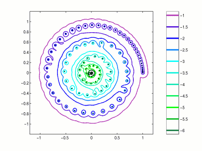
This figure illustrates approximate pseudospectra of an integral equation from laser theory investigated by Landau [Lan77] in one of the earliest applications of pseudospectra. This example discretizes the infinite dimensional problem into a matrix of dimension N=600, and then projects this discretization onto an interesting invariant subspace of dimension 109.

Use the following MATLAB code compute a similar image using EigTool. To mimic the example above, set F=64 and N=600 below.

  F = 12; N = 120;

  % calculate nodes and weights for Gaussian quadrature
  beta = 0.5*(1-(2*[1:N-1]).^(-2)).^(-0.5);
  T = diag(beta,1) + diag(beta,-1);
  [V D] = eig(T); [nodes index] = sort(diag(D));
  weights = zeros(N,1); weights([1:N]) = (2*V(1,index).^2);

  % Construct matrix B
  B = zeros(N,N);
  for k=1:N
    B(k,:)= weights(:)'* sqrt(1i*F).*exp(-1i*pi*F*(nodes(k) - nodes(:)').^2);
  end

  % Weight matrix with Gaussian quadrature weights
  w = sqrt(weights);
  for j=1:N, B(:,j) = w.*B(:,j)/w(j); end
  clear D T V beta index j k nodes w weights

  % Compute Schur form and compress to interesting subspace:
  [U,T] = schur(B); eigB = diag(T);
  select = find(abs(eigB)>.01);
  n = length(select);
  for i = 1:n
    for k = select(i)-1:-1:i
      G([2 1],[2 1]) = planerot([T(k,k+1) T(k,k)-T(k+1,k+1)]')';
      J = k:k+1; T(:,J) = T(:,J)*G; T(J,:) = G'*T(J,:);
    end
  end
  T = triu(T(1:n,1:n));

  opts.npts=50;
  opts.ax = [-1 1.2 -.9 1.1];
  opts.levels = -6:.5:-1;
  eigtool(T,opts)