Worksheet 8: Turtle graphics

This worksheet introduces a different way of drawing pictures that will allow us to escape from the world where every non-trivial picture consists of two other pictures put either one beside the other or one above the other. Instead of joining together tiles, we will give instructions to an imaginary robot called a turtle, telling it whether to turn to the right or left, or go straight on. We will write programs that produce the instructions for the robot as a list y, then use a function turtle(y) that is provided by GeomLab: this function takes the list of instructions and produces a picture of the track that the robot follows.

The turtle obeys a number of different commands, and among them are ahead(x), an instruction to move ahead by x units; left(a), an instruction to turn to the left through an angle of a degrees, and right(a), a similar instruction to turn to the right. When the robot turns, it moves along the arc of a circle that has diameter 1 unit.

The turtle function takes instructions and produces a picture. Its input is not just a single instruction, but a list of instructions that are followed one after another. Lists in the GeomLab language are written with square brackets, so that [left(180), right(90), ahead(1)] is a list of instructions, and supplying it to the turtle function gives the corresponding picture:

turtle([left(180), right(90), ahead(1)])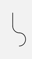

The turtle that follows the list of commands always starts pointing to the right; the starting position is in the middle of the bottom of the picture here. The commands say to turn to the left through a half-circle, then to the right through 90 degrees, then to go straight ahead for 1 unit, and the picture is what results from following these instructions.

GeomLab follows the motion of the turtle as it draws the picture, and makes the picture as large as will fit in the window. Depending on how the turtle moves, the starting and ending positions can be anywhere within the window or at its edge.

GeomLab provides a number of operations that act on lists. If xs and ys are lists, then xs ++ ys is a list that contains all the elements of xs, followed by all the elements of ys. Here's an example that uses lists of numbers instead of lists of commands:

[1, 2, 3] ++ [4, 5] = [1, 2, 3, 4, 5]

Another operation that is provided is reverse, which gives a list that contains the same elements as its argument, but in reverse order:

reverse([1, 2, 3]) = [3, 2, 1]

If xs is a list of commands, then opposite(xs) is a list that is modified so that each command left(a) is replaced by right(a), and vice versa:

opposite([left(90), right(90), left(180), ahead(1)])
  = [right(90), left(90), right(180), ahead(1)]

Here is an example that shows the effect of reversing a list of commands:

turtle(reverse([left(180), right(90), ahead(1)]))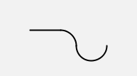

As you can see, the picture us different from the previous one. The function opposite gives a picture that is different again:

turtle(opposite([left(180), right(90), ahead(1)]))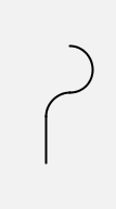

What happens if we apply first reverse and then opposite to a list of commands?

We can use turtle to replicate the Hilbert curves that we drew in Worksheet~7, but describing them now in terms of the turns to left and right that the turtle must make as it follows the curve. The best way to do this is to define a function hilb(n) that produces the list of commands that must be obeyed in drawing the n'th curve in the sequence. Here are the first three curves, drawn in this way:

turtle(hilb(1))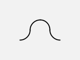

turtle(hilb(2))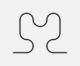

turtle(hilb(3))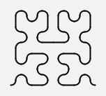

GeomLab draws these curves with smooth turns rather than sharp bends, giving a different effect from the tiled pictures we drew earlier.

To reproduce these results yourself, you will need to define the function hilb that generates the list of commands. For example,

hilb(2) = [ahead(1), left(90), left(90), right(90), ahead(1), 
  right(90), right(90), left(90), left(90), right(90), 
  right(90), ahead(1), right(90), left(90), left(90), ahead(1)]

Each of the curves starts in the bottom left-hand corner of the picture, because the turtle can then start off pointing to the right.

The first six dragon curves look like this:

turtle(dragon(1))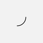

turtle(dragon(2))

turtle(dragon(3))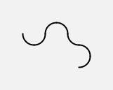

turtle(dragon(4))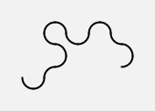

turtle(dragon(5))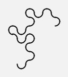

turtle(dragon(6))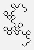

Each successive curve consists of two copies of the preceding curve with a left turn between them; but the second copy is reversed, so that the turtle traces it from what was the end to what was the beginning.

An entertaining way of generating the dragon curve by hand is as follows: take a narrow strip of paper and lay it horizontally in front of you. Take the left-hand end of the strip and lay it over the right-hand end, thus folding the strip in half. Repeat this, taking the crease that is now at the left-hand end and placing it over the right-hand end, folding the strip in half again. Do this several times more, then open out the strip and make each crease into a right-angle. The edge of the strip will then form a dragon curve.

A different, but related, curve can be formed if, instead of performing all the folds from left to right, you alternate between folding the left end over the right and folding the right end over the left. Can you draw this curve with GeomLab?