I come from the Cambridge machine learning group. More than once I heard people referring to us as "the most Bayesian machine learning group in the world". I mean, we do work with probabilistic models and uncertainty on a daily basis. Maybe that's why it felt so weird playing with those deep learning models (I know, joining the party very late). You see, I spent the last several years working mostly with Gaussian processes, modelling probability distributions over functions. I'm used to uncertainty bounds for decision making, in a similar way many biologists rely on model uncertainty to analyse their data. Working with point estimates alone felt weird to me. I couldn't tell whether the new model I was playing with was making sensible predictions or just guessing at random. I'm certain you've come across this problem yourself, either analysing data or solving some tasks, where you wished you could tell whether your model is certain about its output, asking yourself "maybe I need to use more diverse data? or perhaps change the model?". Most deep learning tools operate in a very different setting to the probabilistic models which possess this invaluable uncertainty information, as one would believe. Myself? I recently spent some time trying to understand why these deep learning models work so well – trying to relate them to new research from the last couple of years. I was quite surprised to see how close these were to my beloved Gaussian processes. I was even more surprised to see that we can get uncertainty information from these deep learning models for free – without changing a thing.

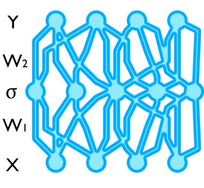
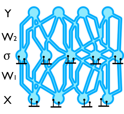
A neural network (a deep learning tool) linearly transforms its input (bottom layer), applies some non-linearity on each dimension (middle layer), and linearly transforms it again (top layer). This model gives us point estimates with no uncertainty information.

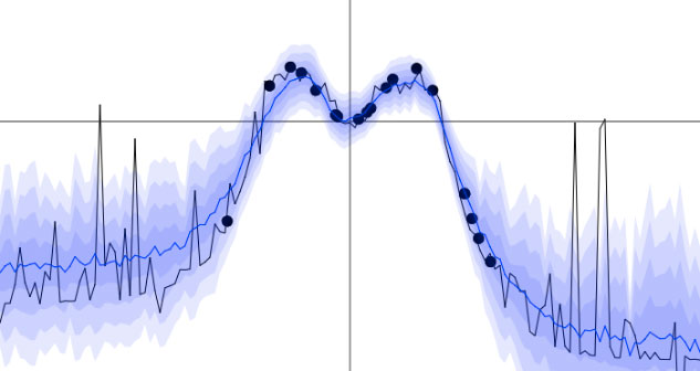
This is what the uncertainty we'll get looks like. We'll play with this interactive demo below.

Update (29/09/2015): I spotted a typo in the calculation of $\tau$; this has been fixed below. If you use the technique with small datasets you should get much better uncertainty estimates now! Also, I added new results to the arXiv paper (Gal and Ghahramani) comparing dropout's uncertainty to the uncertainty of other popular techniques.

Why should I care about uncertainty?

If you give me several pictures of cats and dogs – and then you ask me to classify a new cat photo – I should return a prediction with rather high confidence. But if you give me a photo of an ostrich and force my hand to decide if it's a cat or a dog – I better return a prediction with very low confidence. Researchers use this sort of information all the time in the life sciences (for example have a look at the Nature papers published by Krzywinski and Altman, Herzog and Ostwald, Nuzzo, the entertaining case in Woolston, and the very recent survey by my supervisor Ghahramani). In such fields it is quite important to say whether you are confident about your estimate or not. For example, if your physician advises you to use certain drugs based on some analysis of your medical record, they better know if the person analysing it is certain about the analysis result or not.

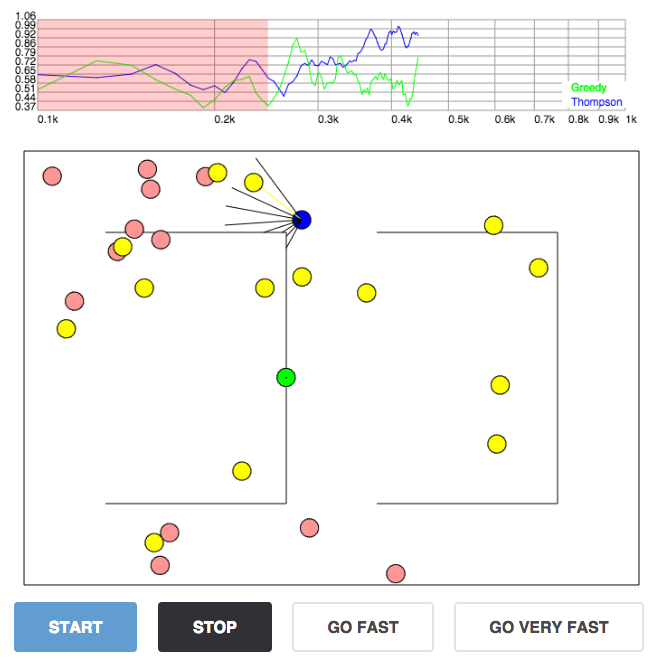
Deep reinforcement learning example: a Roomba navigating within a room; we'll play with this interactive demo below as well.

Uncertainty information is also important for the practitioner. You might use deep learning models on a daily basis to solve different tasks in vision or linguistics. Understanding if your model is under-confident or falsely over-confident can help you get better performance out of it. We'll see below some simplified scenarios where model uncertainty increases far from the data. Recognising that your test data is far from your training data you could easily augment the training data accordingly.

Ok, how can I get this uncertainty information?

For some of these problems above Bayesian techniques would have been used traditionally. And for these problems researchers have recently shifted to deep learning techniques. But this had to come with a cost. I mean, how can you get model uncertainty out of these deep learning tools? (by the way, using softmax to get probabilities is actually not enough to obtain model uncertainty – we'll go over an example below). Well, it's long been known that these deep tools can be related to Gaussian processes, the ones I mentioned above. Take a neural network (a recursive application of weighted linear functions followed by non-linear functions), put a probability distribution over each weight (a normal distribution for example), and with infinitely many weights you recover a Gaussian process (see Neal or Williams for more details). For a finite number of weights you can still get uncertainty by placing distributions over the weights. This was originally proposed by MacKay in 1992, and extended by Neal in 1995 (update: following Yann LeCun's comment below I did some more digging into the history of these ideas; Denker and LeCun have already worked on such ideas in 1991, and cite Tishby, Levin, and Solla from 1989 which place distributions over networks' weights, in which they mention they extend on the ideas suggested in Denker, Schwartz, Wittner, Solla, Howard, Jackel, and Hopfield from 1987, but I didn't go over the book in depth). More recently these ideas have been resurrected under different names with variational techniques by Graves in 2011, Kingma et al. and Blundell et al. from DeepMind in 2015 (although these techniques used with Bayesian neural networks can be traced back as far as Hinton and van Camp dating 1993 and Barber and Bishop from 1998). But these models are very difficult to work with – often requiring many more parameters to optimise – and haven't really caught-on.

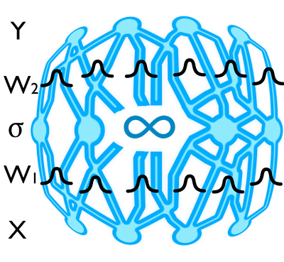
A network with infinitely many weights with a distribution on each weight is a Gaussian process. The same network with finitely many weights is known as a Bayesian neural network. Using these is quite difficult though, and they haven't really caught-on. Or so you'd think.

I think that's why I was so surprised that dropout – a ubiquitous technique that's been in use in deep learning for several years now – can give us principled uncertainty estimates. Principled in the sense that the uncertainty estimates basically approximate those of our Gaussian process. Take your deep learning model in which you used dropout to avoid over-fitting – and you can extract model uncertainty without changing a single thing. Intuitively, you can think about your finite model as an approximation to a Gaussian process. When you optimise your objective, you minimise some "distance" (KL divergence to be more exact) between your model and the Gaussian process. I'll explain this in more detail below. But before this, let's recall what dropout is and introduce the Gaussian process quickly, and look at some examples of what this uncertainty obtained from dropout networks looks like.

Deep models, Dropout, and Gaussian processes

If you feel confident with dropout and Gaussian processes you can safely skip to the next section in which we will learn how to extract the uncertainty information out of dropout networks, and play with the uncertainty we get from neural networks, convolutional neural networks, and deep reinforcement learning. But to get everyone on equal ground let's go over each concept quickly.

Dropout and Deep models

$ \newcommand{\R}{\mathbb{R}} \newcommand{\N}{\mathcal{N}} \newcommand{\cL}{\mathcal{L}} \newcommand{\cO}{\mathcal{O}} \newcommand{\svert}{~|~} \newcommand{\td}{\text{d}} \newcommand{\f}{\mathbf{f}} \newcommand{\x}{\mathbf{x}} \newcommand{\Bb}{\mathbf{b}} \newcommand{\sBb}{\mathtt{b}} \newcommand{\bx}{\overline{\x}} \newcommand{\bb}{\overline{b}} \newcommand{\y}{\mathbf{y}} \newcommand{\z}{\mathbf{z}} \newcommand{\w}{\mathbf{w}} \newcommand{\W}{\mathbf{W}} \newcommand{\ba}{\mathbf{a}} \newcommand{\m}{\mathbf{m}} \newcommand{\ls}{\mathbf{l}} \newcommand{\bL}{\mathbf{L}} \newcommand{\A}{\mathbf{A}} \newcommand{\X}{\mathbf{X}} \newcommand{\Y}{\mathbf{Y}} \newcommand{\F}{\mathbf{F}} \newcommand{\I}{\mathbf{I}} \newcommand{\M}{\mathbf{M}} \newcommand{\p}{\mathbf{p}} \newcommand{\bp}{\overline{\p}} \newcommand{\bz}{\mathbf{0}} \newcommand{\bepsilon}{\text{$\epsilon$}} \newcommand{\bgamma}{\text{$\gamma$}} \newcommand{\s}{\mathbf{s}} \newcommand{\Unif}{\text{Unif}} \newcommand{\bo}{\text{$\omega$}} \newcommand{\bsigma}{s} \newcommand{\bSigma}{\text{$\Sigma$}} \newcommand{\bmu}{\text{$\mu$}} \newcommand{\bphi}{\text{$\phi$}} \newcommand{\K}{\mathbf{K}} \newcommand{\Kh}{\widehat{\mathbf{K}}} \newcommand{\Cov}{\text{Cov}} \newcommand{\Var}{\text{Var}} \newcommand{\tr}{\text{tr}} \newcommand{\tdet}{\text{det}} \newcommand{\diag}{\text{diag}} \newcommand{\KL}{\text{KL}} \newcommand{\ind}{\mathds{1}} \newcommand{\bc}{\mathbf{c}} \newcommand{\reg}{\eta} \newcommand{\wd}{\lambda} \newcommand{\argmin}{\text{argmin}} $

Let's go over the dropout network model quickly for a single hidden layer and the task of regression. We denote by $\W_1, \W_2$ the weight matrices connecting the first layer to the hidden layer and connecting the hidden layer to the output layer respectively. These linearly transform the layers' inputs before applying some element-wise non-linearity $\sigma(\cdot)$. We denote by $\Bb$ the biases by which we shift the input of the non-linearity. We assume the model outputs $D$ dimensional vectors while its input is $Q$ dimensional vectors, with $K$ hidden units. We thus have $\W_1$ is a $Q \times K$ matrix, $\W_2$ is a $K \times D$ matrix, and $\Bb$ is a $K$ dimensional vector. A standard network would output $\widehat{\y} = \sigma(\x \W_1 + \Bb) \W_2$ given some input $\x$.

Dropout is a technique used to avoid over-fitting in these simple networks – a situation where the model can't generalise well from its training data to the test data. It was introduced several years ago by Hinton et al. and studied more extensively in (Srivastava et al.). To use dropout we sample two binary vectors $\sBb_1, \sBb_2$ of dimensions $Q$ and $K$ respectively. The elements of vector $\sBb_i$ take value 1 with probability $0 \le p_i \le 1$ for $i = 1,2$. Given an input $\x$, we set $1 - p_1$ proportion of the elements of the input to zero: $\x \sBb_1$ (to keep notation clean we will write $\sBb_1$ when we mean $\diag(\sBb_1)$ with the $\diag(\cdot)$ operator mapping a vector to a diagonal matrix whose diagonal is the elements of the vector). The output of the first layer is given by $\sigma(\x \sBb_1 \W_1 + \Bb)$, in which we randomly set $1 - p_2$ proportion of the elements to zero, and linearly transform to give the dropout model's output $\widehat{\y} = \sigma(\x \sBb_1 \W_1 + \Bb) \sBb_2 \W_2$. We repeat this for multiple layers.

Dropout is applied by simply dropping-out units at random with a certain probability during training.

To use the network for regression we might use the euclidean loss, $ E = \frac{1}{2N} \sum_{n=1}^N ||\y_n - \widehat{\y}_n||^2_2 $ where $\{\y_1, ..., \y_N\}$ are $N$ observed outputs, and $\{\widehat{\y}_1, ..., \widehat{\y}_N\}$ are the outputs of the model with corresponding observed inputs $\{ \x_1, ..., \x_N \}$. During optimisation a regularisation term is often added. We often use $L_2$ regularisation weighted by some weight decay $\wd$ (alternatively, the derivatives might be scaled), resulting in a minimisation objective (often referred to as cost), \begin{align*} \label{eq:L:dropout} \cL_{\text{dropout}} := E + \wd \big( &||\W_1||^2_2 + ||\W_2||^2_2 \notag\\ &+ ||\Bb||^2_2 \big). \end{align*} Note that optimising this objective is equivalent to scaling the derivatives of the cost by the learning rate and the derivatives of the regularisation by the weight decay after back-propagation, and this is how this optimisation is often implemented. We sample new realisations for the binary vectors $\sBb_i$ for every input point and every forward pass thorough the model (evaluating the model's output), and use the same values in the backward pass (propagating the derivatives to the parameters to be optimised $\W_1,\W_2,\Bb$). The dropped weights $\sBb_1\W_1$ and $\sBb_2\W_2$ are often scaled by $\frac{1}{p_i}$ to maintain constant output magnitude. At test time we do not sample any variables and simply use the full weights matrices $\W_1,\W_2,\Bb$. This model can easily be generalised to multiple layers and classification. There are many open source packages implementing this model (such as Pylearn2 and Caffe).

Gaussian processes

The Gaussian process is a powerful tool in statistics that allows us to model distributions over functions. It has been applied in both the supervised and unsupervised domains, for both regression and classification tasks (Rasmussen and Williams, Titsias and Lawrence). The Gaussian process offers nice properties such as uncertainty estimates over the function values, robustness to over-fitting, and principled ways for hyper-parameter tuning. Given a training dataset consisting of $N$ inputs $\{ \x_1, ..., \x_N \}$ and their corresponding outputs $\{\y_1, ..., \y_N\}$, we would like to estimate a function $\y = \f(\mathbf{x})$ that is likely to have generated our observations. To keep notation clean, we denote the inputs $\X \in \R^{N \times Q}$ and the outputs $\Y \in \R^{N \times D}$.

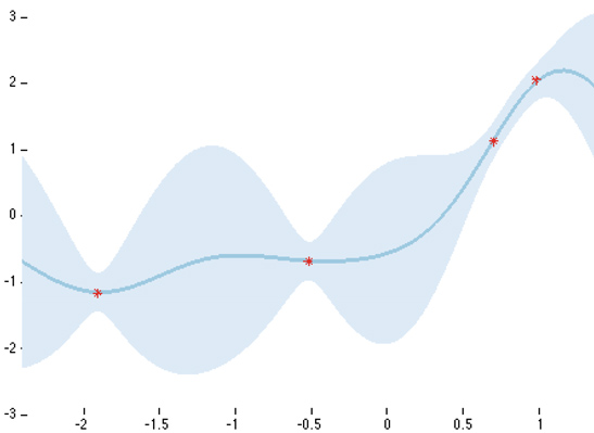
This is what a Gaussian process posterior looks like with 4 data points and a squared exponential covariance function. The bold blue line is the predictive mean, while the light blue shade is the predictive uncertainty (2 standard deviations). The model uncertainty is small near the data, and increases as we move away from the data points.

By modelling our distribution over the space of functions with a Gaussian process we can analytically evaluate its corresponding posterior in regression tasks, and estimate the posterior in classification tasks. In practice what this means is that for regression we place a joint Gaussian distribution over all function values, \begin{align*} \label{eq:generative_model_reg} \F \svert \X &\sim \N(\bz, \K(\X, \X)) \\ \Y \svert \F &\sim \N(\F, \tau^{-1} \I_N) \notag \end{align*} with some precision hyper-parameter $\tau$ and where $\I_N$ is the identity matrix with dimensions $N \times N$.

To model the data we have to choose a covariance function $\K(\X, \X)$ for the Gaussian distribution. This function defines the similarity between every pair of input points $\K(\mathbf{x}_i, \mathbf{x}_j)$. Given a finite dataset of size $N$ this function induces an $N \times N$ covariance matrix $\K := \K(\X, \X)$. This covariance represents our prior belief as to what the model uncertainty should look like. For example we may choose a stationary squared exponential covariance function, for which model uncertainty increases far from the data. Certain non-stationary covariance functions correspond to TanH (hyperbolic tangent) or ReLU (rectified linear) non-linearities. We will see in the examples below what uncertainty these capture. If you want to know how these correspond to the Gaussian process, this is explained afterwards.

Fun with uncertainty^fun

Ok. Let's have some fun with our dropout networks' uncertainty. We'll go over some cool examples of regression and image classification, and in the next section we'll play with deep reinforcement learning. But we still didn't talk about how to get the uncertainty information out of our dropout networks... Well, that's extremely simple.

Take any network trained with dropout and some input $\x^*$. We're looking for the expected model output given our input — the predictive mean $\mathbb{E} (\y^*)$ — and how much the model is confident in its prediction — the predictive variance $\Var \big( \y^* \big)$. As we'll see below, our dropout network is simply a Gaussian process approximation, so in regression tasks it will have some model precision (the inverse of our assumed observation noise). How do we get this model precision? (update: I spotted a typo in the calculation of $\tau$; this has now been fixed) First, define a prior length-scale $l$. This captures our belief over the function frequency. A short length-scale $l$ corresponds to high frequency data, and a long length-scale corresponds to low frequency data. Take the length-scale squared, and divide it by the weight decay. We then scale the result by half the dropout probability over the number of data points. Mathematically this results in our Gaussian process precision $\tau = \frac{l^2 p}{2 N \wd}$ we talked about above (want to see why? go over the section Why does it even make sense? below). Note that $p$ here is the probability of the units not being dropped — in most implementations $p_{\text{code}}$ is defined as the probability of the units to be dropped, thus $p:=1-p_{\text{code}}$ should be used when calculating $\tau$. Next, simulate a network output with input $\x^*$, treating dropout as if we were using it during training time. By that I mean simply drop-out random units in the network at test time. Repeat this several times (say for $T$ repetitions) with different units dropped every time, and collect the results $\{ \widehat{\y}_t^*(\x^*) \}$. These are empirical samples from our approximate predictive posterior. We can get an empirical estimator for the predictive mean of our approximate posterior as well as the predictive variance (our uncertainty) from these samples. We simply follow these two simple equations: \begin{align*} \mathbb{E} (\y^*) &\approx \frac{1}{T} \sum_{t=1}^T \widehat{\y}_t^*(\x^*) \\ \Var \big( \y^* \big) &\approx \tau^{-1} \I_D \\ &\quad+ \frac{1}{T} \sum_{t=1}^T \widehat{\y}_t^*(\x^*)^T \widehat{\y}_t^*(\x^*) \\ &\quad- \mathbb{E} (\y^*)^T \mathbb{E} (\y^*) \end{align*} The first equation was given before in (Srivastava et al.). There it was introduced as model averaging, and it was explained that scaling the weights at test time without dropout gives a reasonable approximation to this equation. This claim was supported by an empirical evaluation. In the next blog post we will see that for some networks (such as convolutional neural networks) this approximation is not sufficient, and can be improved considerably. The second equation is simply the sample variance of $T$ forward passes through the network plus the inverse model precision. Note that the vectors above are row vectors, and that the products are outer-products.

As you'd expect, it is as easy to implement these two equations. We can use the following few lines of Python code to get the predictive mean and uncertainty:

probs = []
for _ in xrange(T):
    probs += [model.output_probs(input_x)]
predictive_mean = numpy.mean(prob, axis=0)
predictive_variance = numpy.var(prob, axis=0)
tau = l**2 * (1 - model.p) / (2 * N * model.weight_decay)
predictive_variance += tau**-1

Let's have a look at this uncertainty for a simple regression problem.

A simple interactive demo

What does our dropout network uncertainty look like? That's an important question, as different network structures and different non-linearities would correspond to different prior beliefs as to what we expect our uncertainty to look like. This property is shared with the Gaussian process as well. Different Gaussian process covariance functions would result in different uncertainty estimates.

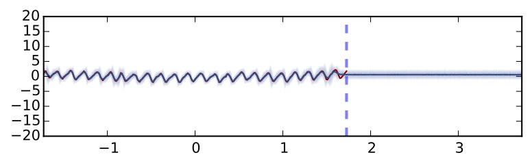
Below is a simple demo (extending on Karpathy's deep learning JavaScript framework) that performs regression with a tiny dropout network. We use 2 hidden layers with 20 ReLU units and 20 sigmoid units, and dropout with probability $0.05$ (as the network is really small) before every weight layer. After every mini-batch update we evaluate the network on the entire space. We plot the current stochastic forward pass through the dropout network (black line), as well as the average of the last 100 stochastic forward passes (predictive mean, blue line) as we learn. Shades of blue denote half a predictive standard deviation for our estimate. You can find the code for this demo here.

Now that we have a feeling as to what the uncertainty looks like, we can perform some simple regression experiments to examine the properties of our uncertainty estimate with different networks and different tasks. We'll extend on this to classification and deep reinforcement learning in the following sections.

Understanding our models

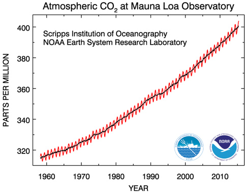
This is what the CO$_2$ dataset looks like before pre-processing.

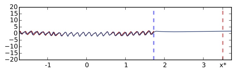
Standard dropout network without using uncertainty information (5 hidden layers, ReLU non-linearity)

The point marked with a dashed red line is a point far away from the training data. I hope you would agree with me that a good model when asked about point $x^*$ should probably say "if you force my hand I'll guess X, but actually I have no idea what's going on". Standard dropout confidently predicts a clearly insensible value for the point — as the function is periodic. We can't really tell whether we can trust the model's prediction or not. Now let's use the uncertainty information equations we introduced above. Using exactly the same network (we don't have to re-train the model, just perform predictions in a different way) we get the following revealing information:

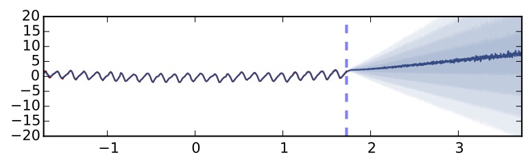
Exactly the same dropout network performing predictions using uncertainty information and predictive mean (5 hidden layers, ReLU non-linearity). Each shade of blue represents half a standard deviation predictive uncertainty.

Gaussian process with SE covariance function on the same dataset

We got a different uncertainty estimate that still increases far from the data. It is not surprising that the uncertainty looks different — the ReLU non-linearity corresponds to a different Gaussian process covariance function. What would happen if we were to use a different non-linearity (i.e. a different covariance function)? Let's try a TanH non-linearity:

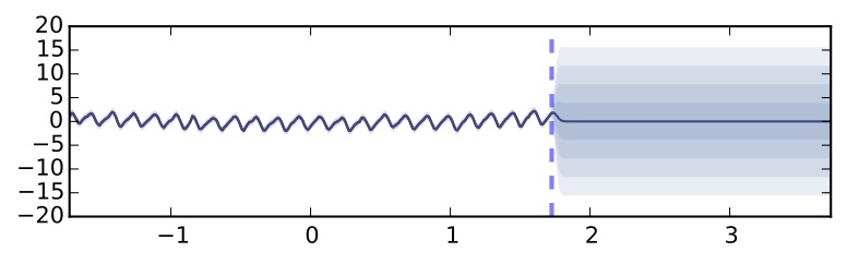
Dropout network using uncertainty information and TanH non-linearity (5 hidden layers)

It seems that the uncertainty doesn't increase far from the data... This might be because TanH saturates whereas ReLU does not. This non-linearity will not be appropriate for tasks where you'd expect your uncertainty to increase as you go further away from the data.

What about different network architectures or different dropout probabilities? For the TanH model I tested the uncertainty using both dropout probability $0.1$ and dropout probability $0.2$. The models initialised with dropout probability $0.1$ initially do show smaller uncertainty than the ones initialised with dropout probability $0.2$, but towards the end of the optimisation, when the model has converged, the uncertainty is almost undistinguishable. It also seems that using a smaller number of layers doesn't affect the resulting uncertainty — experimenting with 4 hidden layers instead of 5 hidden layers there was no significant difference in the results. As a side note, it's quite funny to mention that it took me 5 minutes to get the Gaussian process to fit the dataset above, and 3 days for the dropout networks. But that's probably just because I've never worked with these models before, and none of my Gaussian process intuition carried over to the multiple layers case. Also, a single hidden layer network works just as well, sharing many characteristics with the shallow Gaussian process.

This is what the solar irradiance dataset looks like before pre-processing (in brown).

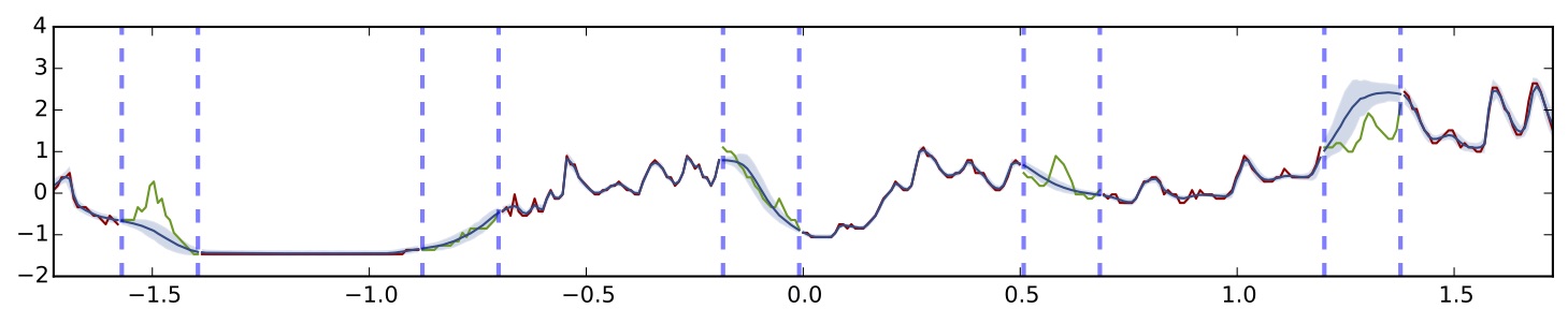
Gaussian process with SE covariance function

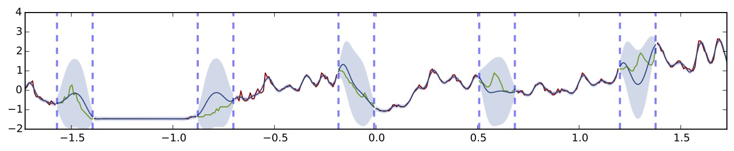
Again, the observed function is given in red, with missing sections given in green. In blue is the model's prediction both on the observed subsets and missing subsets. In light blue is predictive uncertainty with 2 standard deviations. It seems that the model manages to capture the function very well with with increased uncertainty over the missing sections. Let's see what a dropout network looks like on this dataset. We'll use the same network structure as before with 5 hidden layers and ReLU non-linearities:

Dropout network using uncertainty information on the same dataset (5 hidden layers, ReLU non-linearity)

It seems that the model fits the data very well as well, but with smaller model uncertainty. This is actually a well known limitation of variational approximations. As dropout can be seen as a variational approximation to the Gaussian process, this is not surprising at all. It is possible to correct this under-estimation of the variance and I will write another post about this in the coming future.

Image Classification

Let's look at a more interesting example — image classification. We'll classify MNIST digits (LeCun and Cortes) using the popular LeNet convolutional neural network (LeCun et al.). In this model we feed our prediction into a softmax which gives us probabilities for the different classes (the 10 digits). Interestingly enough, these probabilities are not enough to see if our model is certain in its prediction or not. This is because the standard model would pass the predictive mean through the softmax rather than the entire distribution.

Let's look at an idealised binary classification example. Passing a point estimate of the mean of a function (a TanH function for simplicity, solid line on the left in the figure below) through a softmax (solid line on the right in the figure below) results in highly confident extrapolations with $x^*$ (a point far from the training data) classified as class $1$ with probability $1$. However, passing the distribution (shaded area on the left) through a softmax (shaded area on the right) reflects classification uncertainty better far from the training data. Taking the mean of this distribution passed through the softmax we get class $1$ with probability $0.5$ — the model's true prediction.

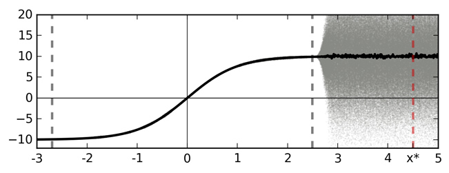
Softmax input as a function of data $\x$

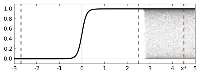
Softmax output as a function of data $\x$

A sketch of softmax input and output for an idealised binary classification problem. Training data is given between the dashed grey lines. Function point estimate is shown with a solid line (TanH for simplicity — left). Function uncertainty is shown with a shaded area. Marked with a dashed red line is a point $x^*$ far from the training data. Ignoring function uncertainty, point $x^*$ is classified as class 1 with probability 1.

Ok, so let's pass the entire distribution through the softmax instead of the mean alone. This is actually very easy — we just simulate samples through the network and average the softmax output. Let's evaluate our convnet trained over MNIST with dropout applied after the last inner-product layer (with probability 0.5 as the network is fairly large). We'll evaluate model predictions over the following sequence of images, that correspond to some projection in the image space:

Image inputs (a rotated digit) to our dropout LeNet network

These images correspond to our $X$ axis in the idealised depiction above. Let's visualise the histogram of 100 samples we obtain by simulating forward passes through our dropout LeNet network:

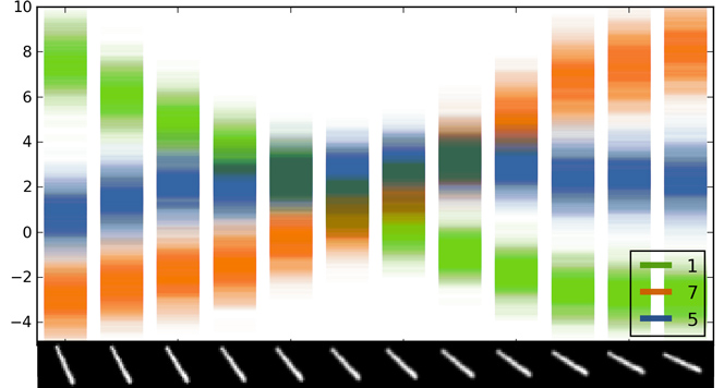
Softmax input scatter

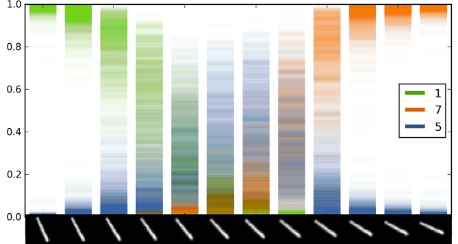
Softmax output scatter

A scatter of 100 forward passes of the softmax input and output for dropout LeNet. On the $X$ axis is a rotated image of the digit 1. The input is classified as digit 5 for images 6-7, even though model uncertainty is extremly large.

Class 7 has low uncertainty for the right-most images. This is because the uncertainty ``envelope'' of the softmax input for these images is far away from the uncertainty envelopes of all other classes. In contrast, the uncertainty envelope of class 5 for the middle images intersects the envelopes of some of the other classes (even though it's mean is higher) — resulting in large uncertainty for the softmax output. It is important to note that the model uncertainty in the softmax output can be summarised by taking the mean of the distribution. In the idealised example above this would result in softmax output $0.5$ for point $x^*$ (instead of softmax output $1$) and here it will result in a lower softmax output that might result in a different image class. This sort of information can help us in classification tasks — obtaining higher classification accuracies as will be explained in the next blog post. It also helps us analyse our model and decide whether we have enough data or if the model is specified correctly.

Uncertainty in deep reinforcement learning

Let's do something more exciting with our uncertainty information. We can use this information for deep reinforcement learning, where we use a network to learn what actions an independent agent (for example a Roomba or a humanoid robot) should take to solve a given task (for example clean your apartment or eliminate humanity). In reinforcement learning we get rewards for different actions, for example a $-5$ reward for walking into a wall and a $+10$ reward for collecting food (or dirt if you're a Roomba). However our environment can be stochastic and ever changing. We want to maximise our expected reward over time, basically learn what actions are appropriate in different situations. For example, if I see food in front of me I should go forward rather than go left. We do this by exploring our environment, ideally minimising our uncertainty about rewards resulting from different states and actions we take.

Recent research from DeepMind (a blue skies research company acquired by Google a couple of years ago), through heavy engineering efforts, managed to demonstrate human level game playing of various Atari games. They used a neural network to control what actions the agent should take in different states (Mnih et al.). This approach is believed by some to be a starting point towards solving AI. This work by DeepMind extends on several existing approaches in the field (for example see neural fitted Q-learning by Riedmiller). However no agent uncertainty is modelled with this approach, and an epsilon-greedy behavioural policy is used instead (taking random actions with probability $\epsilon$ and optimal actions otherwise). Gaussian processes have been used in the past to represent agent uncertainty, but did not scale well beyond simple toy problems (see PILCO for example, Deisenroth and Rasmussen). Regarding our dropout network as a Gaussian process approximation we can use its uncertainty estimates for the same task without any additional cost.

Our deep reinforcement learning setting.

At every point in time the agent evaluates its belief as to the quality of all possible actions it can take in its current state (denoted as the $Q$-function), and then proceeds to take the action with the highest value. This $Q$-function captures the agent's subjective belief of the value of a given state $s$. This value is defined as the expected reward over time resulting from taking action $a$ at state $s$, with the expectation being with respect to the agent's current understanding of how the world works (you can read more about reinforcement learning in this very nice book by Szepesvári). We use ``replay'' to train our network — in which we collect tuples of state, action, resulting state, and resulting reward as training data for the network. We then perform one gradient descent step with a mini-batch composed of a random subset of the collection of tuples.

The behavioural policy used in Mnih et al. and Karpathy's implementation is epsilon-greedy with a decreasing schedule. In this policy the agent starts by performing random actions to collect some data, and then reduces the probability of performing random actions. Instead of performing random actions the agent would evaluate the network's output on the current state and choose the action with the highest value. Now, instead of that we can try to minimise our network's uncertainty. This is actually extremely simple: we just use Thompson sampling (Thompson). Thompson sampling is a behavioural policy that encourages the agent to explore its surrounding by drawing a realisation from our current belief over the world and choosing the action with the highest value following that belief. In our case this is simply done by simulating a stochastic forward pass through the dropout network and choosing the action with the highest value.

If you can't run the JavaScript below (it takes some time to converge...), this is what the average reward over time looks like for both epsilon greedy and Thompson sampling (on log scale):

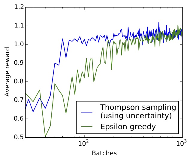
Average reward over time for epsilon greedy (green) and Thompson sampling (blue) on log scale. Thompson sampling converges an order of magnitude faster than epsilon greedy.

Below you'll see the agents learning an appropriate policy over time. For epsilon greedy I use exactly the same implementation as Karpathy's, and for dropout I added a single dropout layer with probability $0.2$ (as the network is fairly small). The top of the plot is a graph showing the average reward on log scale. The first 3000 moves for both agents are random, used to collect initial data before training. This is shown with a red shade in the graph. The algorithm is stochastic, so don't be surprised if sometimes the blue curve (Thompson sampling) goes below the green one (epsilon greedy). Note that the $X$ axis of the graph shows the number of batches divided by $100$. You can find the code for this demo here.

It's interesting to mention that apart from the much faster convergence, using dropout also circumvents over-fitting in the network. But because the network is so small we can't really use dropout properly — after every layer — as the variance would be too large. We'll discuss this in more detail below in diving into the derivation. It's also worth mentioning some difficulties with Thompson sampling. As we sample based on the model uncertainty we might get weird results from under-estimation of the uncertainty. This can be fixed rather easily though and will be explained in a future post. Another difficulty is that the algorithm doesn't distinguish between uncertainty about the world (which is what we care about) and uncertainty resulting from misspecification of our network. So if our network is under-fitting its data, not being able to reduce its uncertainty appropriately, the model will suffer.

Why does it even make sense?

Let's see why dropout neural networks are identical to variational inference in Gaussian processes. We'll see that what we did above, averaging forward passes through the network, is equivalent to Monte Carlo integration over a Gaussian process posterior approximation. The derivation uses some long equations that mess-up the page layout on mobile devices – so I put it here with a toggle to show and hide it easily. Tap here to show the derivation: Derivation Tap here to hide the derivation: Derivation

Diving into the derivation

The derivation above sheds light on many interesting properties of dropout and other ``tricks of the trade'' used in deep learning. Some of these are described in the appendix of (Gal and Ghahramani). Here we'll go over deeper insights arising from the derivation. I'd like to thank Mark van der Wilk for some of the questions raised below.

First, can we get uncertainty estimates over the weights in our dropout network? it might be a bit difficult to see this with the Bernoulli case, so for simplicity imagine that our approximating distribution is a single Gaussian distribution parametrised by its mean and standard deviation. In our variational inference setting we fit the entire distribution to our posterior, trying to approximate it as best we can. This involves optimising over the variational parameters — the mean and the standard deviation. This is standard in variational inference where we fit distributions rather than parameters, resulting in our robustness to over-fitting. The fitted Gaussian distribution captures our uncertainty estimate over the weights. Now, it's the same for the Bernoulli case. Optimising our variational lower bound we are matching the Bernoulli approximate posterior to our true posterior. For comparison, the MAP estimate is obtained when we use a single delta function in our approximating distribution, in which case our integration over the parameters collapses to a single point estimate. Our Bernoulli approximation is a sum of two delta functions, resulting in the averaging of many possible models. The non-zero component in our mixture of Gaussians is the variational parameter we optimise over to fit the distributions. But the Bernoullis are not important at all for this! DropConnect (Wan et al.) or Multiplicative Gaussian Noise (section 10 in Srivastava et al.) follow our interpretation exactly (and are equivalent to alternative approximating distributions). The example above of a single Gaussian can be neatly extended to these. So in short, yes, we can get uncertainty estimates over the features — this is the posterior $q_\theta(\bo)$ above!

Why is the variance estimation of the model sensible? In the mixture of Gaussians approximating distribution (which is used to approximate the Bernoulli distribution) only the mean changes and the variance is fixed, aren't they? That's actually a bit more difficult to see. If we use our approximating distribution recursively in each layer and the architecture is deep enough, the mean of the Gaussians would change to best represent the uncertainty we can't change. This is because we minimise the KL divergence from the full posterior, which would result in the approximating model fitting not just the first moment of the posterior (our predictive mean) but also the second moment (resulting in a sensible variance estimate). That's why optimising the mean alone for our variational distribution, even though we have fixed uncertainty for each single distribution, the model as a whole will approximate the posterior uncertainty the best it can. For the same reason it seems that optimising the dropout probabilities is not that important as long as they are sensible. During optimisation the weight means (our variational parameters) will simply adapt to match the true posterior as far as the model architecture allows it. Although, as mentioned in the appendix of (Gal and Ghahramani), we can also optimise over the dropout probabilities as these are just variational parameters.

It's also quite cool to see that the dropout network, which was developed following empirical experimentation, is equivalent to using a popular variance reduction technique in our Gaussian process approximation above. More specifically, in the full derivation in the appendix of (Gal and Ghahramani), to match the dropout model, we have to re-parametrise the model so the random variables do not depend on any parameters, thus reducing the variance in our Monte Carlo estimator. You can read more about this in Kingma and Welling. This can also explain why dropout under-performs for networks which are small in comparison to dataset size. Presumably the estimator variance is just too large.

The above developments also suggest a new interpretation into why dropout works so well as a regularisation technique. At the moment it is thought in the field that dropout works because of the noise it introduces. I would say that the opposite is true: dropout works despite the noise it introduces!. By that I mean that the noise, interpreted as approximate integration, is a side-effect of integrating over the model parameters. If we could we would evaluate the integrals analytically without introducing this additional noise. Indeed, that's what many approaches to Bayesian neural networks do in practice.

It is also interesting to note that the posterior in the Gaussian process approximation above is not actually a Gaussian process itself. By integrating over the variables $\bo$ (which can also be seen as integrating over a random covariance function) the resulting distribution does not have Gaussian marginals any more. It is conditionally Gaussian however — when we condition on a specific covariance function we get Gaussian marginals. This is also what happens when we put prior distributions over the Gaussian process hyper-parameters or priors over the covariance function, such as a Wishart process prior (Shah et al.). For a Wishart process prior we have analytical marginals, but the resulting distribution is not expressive enough for many applications. Another property of the approximation above, through the integration over the covariance function, is that we actually change the feature space over which the Gaussian process is defined. In normal Gaussian process models we have a fixed feature space given by a deterministic covariance function and only the weights of the different features change a-posteriori. In our case the covariance function is random and has a posterior conditioned on observed data. The Gaussian process feature space thus changes a-posteriori.

What's next

I think future research at the moment should concentrate on better uncertainty estimates for our models above. The fact that we can use Bernoulli approximating distributions to get reasonably good uncertainty estimates helps us in computationally demanding settings, but with alternative approximating distributions we should be able to improve on these uncertainty estimates. Using multiplicative Gaussian noise, multiplying the units by $\N(1,1)$ for example, might result in more accurate uncertainty estimates, and many other similarly expressive yet computationally efficient distributions exist out there. It will be really interesting to see principled and creative use of simple distributions that would result in powerful uncertainty estimates.

Source code

I put the models used with the examples above here so you can play with them yourself. The models use Caffe for both the neural networks and convolutional neural networks. You can also find here the code for the interactive demos using Karpathy's framework.

Conclusions

We saw that we can get model uncertainty from existing deep models without changing a single thing. Hopefully you'll find this useful in your research, be it data analysis in bioinformatics or image classification in vision systems. In the next post I'll go over the main results of Gal and Ghahramani showing how the insights above can be extended to get Bayesian convolutional neural networks, with state-of-the-art results on CIFAR-10. In a future post we'll use model uncertainty for adversarial inputs such as corrupted images that classify incorrectly with high confidence (have a look at intriguing properties of neural networks or breaking linear classifiers on ImageNet for more details). Adding or subtracting a single pixel from each input dimension is perceived as almost unchanged input to a human eye, but can change classification probabilities considerably. In the high dimensional input space the new corrupted image lies far from the data, and model uncertainty should increase for such inputs.

Further Reading

If you'd like to learn more about Gaussian processes you can watch Carl Rasmussen's video lecture, Philipp Hennig's video lectures, or have a look at some notes from past Gaussian process summer schools. You can also go over the Gaussian Processes for Machine Learning book, available online.

I also have several other past projects involving Gaussian processes, such as distributed inference in the Gaussian process with Mark van der Wilk and Carl E. Rasmussen (NIPS 2014), distribution estimation of vectors of discrete variables with stochastic variational inference with Yutian Chen and Zoubin Ghahramani (ICML 2015), variational inference in the sparse spectrum approximation to the Gaussian process with Richard Turner (ICML 2015), and a quick tutorial to Gaussian processes with Mark van der Wilk on arXiv.

Our developments above also show that dropout can be seen as approximate inference in Bayesian neural networks, which I'll explain in more depth in the next post. In the mean time, for interesting recent research on Bayesian neural networks you can go over variational techniques to these (Graves from 2011, Gal and Ghahramani, Kingma et al. and Blundell et al. from 2015), Bayesian Dark Knowledge by Korattikara et al., Probabilistic Backpropagation by Miguel Hernández-Lobato and Ryan Adams, and stochastic EP by Li et al.

Acknowledgements

I'd like to thank Christof Angermueller, Roger Frigola, Shane Gu, Rowan McAllister, Gabriel Synnaeve, Nilesh Tripuraneni, Yan Wu, and Prof Yoshua Bengio and Prof Phil Blunsom for their helpful comments on either the papers or the blog post above or just in general. Special thanks to Mark van der Wilk for the thought-provoking discussions on the approximation properties.

Citations

Do you want to use these results for your research? You can cite Gal and Ghahramani (or download the bib file directly). There are also lots more results in the paper itself.

Discussion