Traditional analysis of linear models is based upon eigenvalues, and for many problems across mathematics, science, and engineering, such analysis is successful. This is most notably true for self-adjoint matrices and operators, which possess a basis of orthogonal eigenvectors. Areas of successful applications of eigenvalue techniques include acoustics, structural analysis, quantum mechanics, low-Reynolds-number fluid mechanics, and numerical analysis.

In recent decades, recognition has grown that one must proceed with greater caution when a matrix or operator lacks an orthogonal basis of eigenvectors. Such operators are called non-normal, and this property can lead to a rich variety of behavior. For example, non-normality can be associated with transient behavior that differs entirely from the asymptotic behavior suggested by eigenvalues. Such transients may manifest themselves in slow convergence of iterative processes, in nearness to instability, and in the transition to turbulence in fluid flow.

Numerous tools have been suggested to describe non-normality and analyze its effects. These include classical tools of matrix and operator theory, such as the numerical range, the angles between invariant subspaces, and the condition numbers of eigenvalues. This web site is devoted to describing and illustrating pseudospectra, a further tool that has proved useful in a variety of circumstances.

Suppose we have a square n-by-n complex matrix,

The eigenvalues of A satisfy the following definition.

If z is an eigenvalue of A, then by convention we define the norm of (zI-A)^-1 to be infinity. But what if ||(zI-A)^-1|| is finite but very large? This pattern of thinking leads to a first definition of pseudospectra.

Equivalently, the epsilon-pseudospectrum can be defined in terms of eigenvalues of perturbed matrices.

If z is in the epsilon-pseudospectrum, it is an epsilon-pseudo-eigenvalue of A. With each pseudo-eigenvalue we can associate a pseudo-eigenvector (non-unique, in general), and these quantities lead to a third definition of pseudospectra.

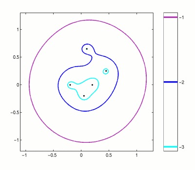
The equivalence of Definitions 1, 2, and 3 is demonstrated on the Theorems page of this web site.

If the matrix or operator A is normal (i.e., it has an orthogonal basis of eigenvectors), then its 2-norm epsilon-pseudospectrum consists of closed balls of radius epsilon surrounding the eigenvalues. For non-normal matrices, the pseudospectra can be much larger, and thus much more interesting.

More generally (in any norm), trouble arises if the basis of eigenvectors is ill-conditioned. If a vector is written in terms of this basis, the expansion coefficients may be huge relative to the size of the vector itself. The "physics" of the system may then be dominated by the evolving pattern of cancellation of these coefficients, rather than by the behavior of individual eigenvalues.

Consider a simple example, the 2-norm pseudospectra of a matrix of dimension five, illustrated in Figure 1. All pseudospectra plots at this web site follow this general template. The eigenvalues are plotted as black dots on the complex plane, and colored lines mark the boundaries of various pseudospectra. The color bar on the right indicates the log₁₀ of each boundary, so in Figure 1 we draw the boundaries of the epsilon-pseudospectra for epsilon = 10^-1, 10^-2, and 10^-3. Notice that for some values of epsilon, the pseudospectrum is connected, while for smaller epsilon it can consist of disjoint sets. Sometimes the pseudospectral boundary about an eigenvalue is too small to be clearly visible on our plots. In Figure 1, this is the case for the 10^-3 contour about the eigenvalue with largest imaginary part.

To view further illustrations of pseudospectra on this web site, begin with the Examples page.

Figure 1. Spectrum (black dots) and boundaries (colored lines) of three epsilon-pseudospectra for a matrix of dimension five.

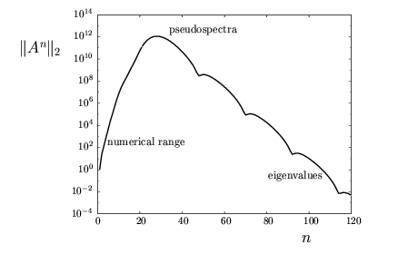
Areas where non-normality is important include: hydrodynamic instability, matrix iterations, meteorology, Markov chains, control theory, and analysis of high-powered lasers. A more detailed list can be found in the Applications section.

We close this introduction with an example of the kind of information that pseudospectra can reveal. The convergence of iterative matrix processes (such as a discretized differential equation or a stationary iterative method for solving a system of linear algebraic equations) can be described in terms of norms of matrix powers. If all the eigenvalues of a matrix are smaller than one in magnitude, then ||Aⁿ|| must eventually converge to zero as n increases. Non-normality can lead to some period of growth before this decay, however. An example of this behavior is shown in Figure 2. Analysis of the transient period can be based on the numerical range and the pseudospectra, as described in [HT93].

Figure 2. Transient growth, followed by eventual decay, of ||An|| for a non-normal matrix. For continuous rather than discrete time, the analogous plot would show ||eAt|| against t.