Uncertainty in Deep Learning
(PhD Thesis)
October 13th, 2016 (Updated: June 4th, 2017)
Function draws from a dropout neural network. This new visualisation technique depicts the distribution over functions rather than the predictive distribution (see demo below).
Thesis: Uncertainty in Deep Learning
Some of the work in the thesis was previously presented in [Gal, 2015; Gal and Ghahramani, 2015a,b,c,d; Gal et al., 2016], but the thesis contains many new pieces of work as well. The most notable of these are
- some discussions: a discussion of AI safety and model uncertainty (§1.3), a historical survey of Bayesian neural networks (§2.2),
- some theoretical analysis: a theoretical analysis of the variance of the re-parametrisation trick and other Monte Carlo estimators used in variational inference (the re-parametrisation trick is not a universal variance reduction technique! §3.1.1–§3.1.2), a survey of measures of uncertainty in classification tasks (§3.3.1),
- some empirical results: an empirical analysis of different Bayesian neural network priors (§4.1) and posteriors with various approximating distributions (§4.2), new quantitative results comparing dropout to existing techniques (§4.3), tools for heteroscedastic model uncertainty in Bayesian neural networks (§4.6),
- some applications: a survey of recent applications in language, biology, medicine, and computer vision making use of the tools presented in this thesis (§5.1), new applications in active learning with image data (§5.2),
- and more theoretical results: a discussion of what determines what our model uncertainty looks like (§6.1–§6.2), an analytical analysis of the dropout approximating distribution in Bayesian linear regression (§6.3), an analysis of ELBO-test log likelihood correlation (§6.4), discrete prior models (§6.5), an interpretation of dropout as a proxy posterior in spike and slab prior models (§6.6, relating dropout to works by MacKay, Nowlan, and Hinton from 1992), as well as a procedure to optimise the dropout probabilities based on the variational interpretation to separate the different sources of uncertainty (§6.7).
- Contents (PDF, 36K)
- Chapter 1: The Importance of Knowing What We Don't Know (PDF, 393K)
- Chapter 2: The Language of Uncertainty (PDF, 136K)
- Chapter 3: Bayesian Deep Learning (PDF, 302K)
- Chapter 4: Uncertainty Quality (PDF, 2.9M)
- Chapter 5: Applications (PDF, 648K)
- Chapter 6: Deep Insights (PDF, 939K)
- Chapter 7: Future Research (PDF, 28K)
- Bibliography (PDF, 72K)
- Appendix A: KL condition (PDF, 71K)
- Appendix B: Figures (PDF, 2M)
- Appendix C: Spike and slab prior KL (PDF, 28K)
One of the nice practical new results in section §4.1 for example affects function visualisation. It's a minor change that has gone unnoticed until now, but which is significant in understanding our functions.
Function visualisation
There are two factors at play when visualising uncertainty in dropout Bayesian neural networks: the dropout masks and the dropout probability of the first layer. Uncertainty depictions in my previous blog posts drew new dropout masks for each test point—which is equivalent to drawing a new prediction from the predictive distribution for each test point $-2 \leq \x \leq 2$. More specifically, for each test point $\x_i$ we drew a set of network parameters from the dropout approximate posterior $\boh_{i} \sim q_\theta(\bo)$, and conditioned on these parameters we drew a prediction from the likelihood $\y_i \sim p(\y | \x_i, \boh_{i})$. Since the predictive distribution has \begin{align*} p&(\y_i | \x_i, \X_\train, \Y_\train) \\ &= \int p(\y_i | \x_i, \bo) p(\bo | \X_\train, \Y_\train) \text{d} \bo \\ &\approx \int p(\y_i | \x_i, \bo) q_\theta(\bo) \text{d} \bo \\ &=: q_\theta(\y_i | \x_i) \end{align*} we have that $\y_i$ is a draw from an approximation to the predictive distribution.
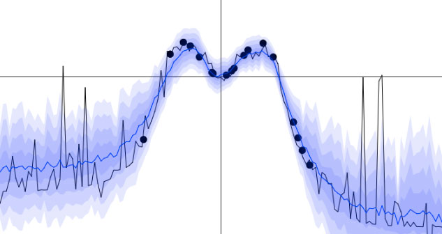
Figure A: In black is a draw from the predictive distribution of a dropout neural network $\yh \sim q_\theta(\y | \x)$ for each test point $-2 \leq \x \leq 2$, compared to the function draws in figure B.
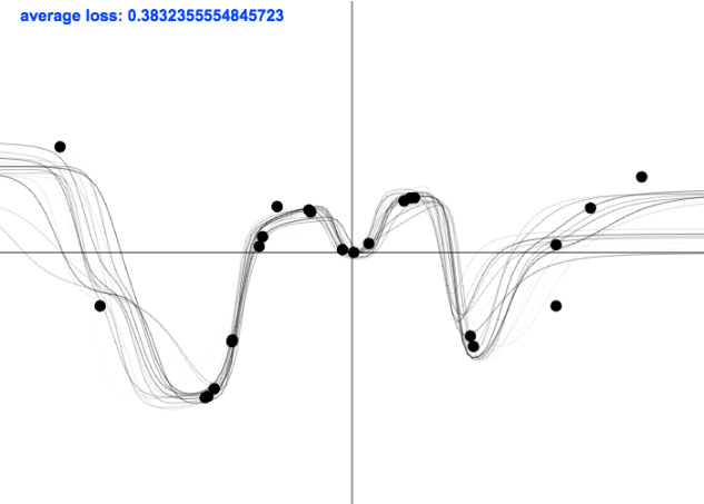
Figure B: Each solid black line is a function drawn from a dropout neural network posterior over functions, induced by a draw from the approximate posterior over the weights $\boh \sim q_\theta(\bo)$.
Another important factor affecting visualisation is the dropout probability of the first layer. In the previous posts we depicted scalar functions and set all dropout probabilities to $0.1$. As a result, with probability $0.1$, the sampled functions from the posterior would be identically zero. This is because a zero draw from the Bernoulli distribution in the first layer together with a scalar input leads the model to completely drop its input (explaining the points where the function touches the $x$-axis in figure A). This is a behaviour we might not believe the posterior should exhibit (especially when a single set of masks is drawn for the entire test set), and could change this by setting a different probability for the first layer. Setting $p_1 = 0$ for example is identical to placing a delta approximating distribution over the first weight layer.
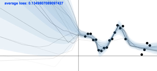
In the demo below we use $p_1 = 0$, and depict draws from the approximate predictive distribution evaluated on the entire test set $q_{\theta_i}(\Y | \X, \boh_i)$ ($\boh_i \sim q_{\theta_i}(\bo)$, function draws), as the variational parameters $\theta_i$ change and adapt to minimise the divergence to the true posterior (with old samples disappearing after 20 optimisation steps). You can change the function the data is drawn from (with two functions, one from the last blog post and one from the appendix in this paper), and the model used (a homoscedastic model or a heteroscedastic model, see section §4.6 in the thesis for example or this blog post).
Last 20 function draws (together with predictive mean and predictive variance) for a dropout neural network, as the approximate posterior is transformed to fit the true posterior. This is done for two functions, both for a homoscedastic model as well as for a heteroscedastic one. You can add new points by left clicking.
Acknowledgements
To finish this blog post I would like to thank the people that helped through comments and discussions during the writing of the various papers composing the thesis above. I would like to thank (in alphabetical order) Christof Angermueller, Yoshua Bengio, Phil Blunsom, Yutian Chen, Roger Frigola, Shane Gu, Alex Kendall, Yingzhen Li, Rowan McAllister, Carl Rasmussen, Ilya Sutskever, Gabriel Synnaeve, Nilesh Tripuraneni, Richard Turner, Oriol Vinyals, Adrian Weller, Mark van der Wilk, Yan Wu, and many other reviewers for their helpful comments and discussions. I would further like to thank my collaborators Rowan McAllister, Carl Rasmussen, Richard Turner, Mark van der Wilk, and my supervisor Zoubin Ghahramani.
Lastly, I would like to thank Google for supporting three years of my PhD with the Google European Doctoral Fellowship in Machine Learning, and Qualcomm for supporting my fourth year with the Qualcomm Innovation Fellowship.
PS. there might be some easter eggs hidden in the introduction :)
Discussion